Updates to Mutation, Randomness and Evolution
Most recent update: 3 November, 2023, initial version. See the change-log at the bottom for details.
This is an ongoing list of updates and corrections to Mutation, Randomness and Evolution, including typographic errors, as well as substantive errors and updates to knowledge.
Typos and glitches
The following mistakes (given in order, by section number) might be confusing or misleading:
- section 1.1 refers 3 times to a “50-fold range” of mutation rates in MacLean, et al (2010), but the actual range is 30-fold.
- section 2.3. See the note about 1.1 (30-fold, not 50-fold)
- in section 4.3, replace “development, growth, and hereditary” with “development, growth, and heredity”
- section 4.5 describes a hypothetical experiment examining 20 mutations each for 5 species, then refers to “our small set of 20 X 10” mutations instead of “our small set of 20 X 5” mutations
- section 5.7, the reference to the “ongoing commitment of evolutionary biologists to neo-Darwinism” is actually refering to the second aspect of neo-Darwinism, i.e., not adaptationism but the dichotomy of roles in which variation is subservient to selection
- Fig 9.7 right panel title refers to “Frequency rate vs. fitness” instead of “Mutation rate vs. fitness”
- section 9.3. See the note about 1.1 (30-fold, not 50-fold)
- section A.3, the equation is mis-formatted. The left-hand side should be xi+1, not xi + 1
More recent work on topics covered in MRE
MRE was mostly completed in 2019 and only has a few citations to work published in 2020. For perspectives more up-to-date, see the following.
- Overviews and summaries of the evidence
- very brief: Misrepresenting biases in arrival (Cano, et al., 2023)
- longer: Mutation bias and the predictability of evolution (Cano, et al, 2023)
- even longer: Bias in the introduction of variation (wikipedia page)
- Overviews and summaries of the theory of arrival bias
- Mutation bias and the predictability of evolution (Cano, et al, 2023)
- Bias in the introduction of variation (wikipedia page)
- Significant new work on arrival bias (some of this is addressed further below)
- Horton and Taylor (2023) Mutation bias and adaptation in bacteria (review)
- Dingle, et al. (2022) Phenotype Bias Determines How Natural RNA Structures Occupy the Morphospace of All Possible Shapes
- Cano, et al. (2022) Mutation bias shapes the spectrum of adaptive substitutions
- Horton, et al (2021) A mutational hotspot that determines highly repeatable evolution can be built and broken by silent genetic changes
- Correcting ongoing misrepresentations by Svensson (2022, 2023)
- Misrepresenting biases in arrival (Cano, et al., 2023)
Specific updates and clarifications
Ch. 8 covers the theory of arrival bias, and Ch. 9 covers evidence. Both chapters suggest generalizations that are subject to further evaluation. Most of the updates are going to involve these two chapters.
Prediction regarding self-organization (MRE 8.11)
For a long time, I’ve been arguing that one sense of “self-organization” in the work of Kauffman (1993) and others is an effect of findability that is related to the explanation for King’s codon argument, arising from biases in the introduction process (Stoltzfus, 2006, 2012). MRE 8.11 calls this “the obvious explanation for the apparent magic of Kauffman’s ‘self-organization'”, and suggests how to demonstrate this directly by implementing an artificial mutation operator that samples equally by phenotype.
This demonstration has been done— independently of my suggestions— by Dingle, et al. (2022), Phenotype Bias Determines How Natural RNA Structures Occupy the Morphospace of All Possible Shapes. The findability of intrinsically likely forms has been explored in an important series of studies from Ard Louis’s group. The earliest one, Schaper and Louis (2014), actually appeared before MRE was finished (I saw it but did not grasp the importance). More recent papers such as Dingle, et al. (2022) have made it clear that the “arrival of the frequent” or “arrival bias” in this work is a reference to biases in the introduction process that favor forms (phenotypes, folds) that are over-represented (i.e., frequent) in genotypic state-space.
A variety of think-pieces have speculated about what is the relationship of self-organization to natural selection (Johnson and Lam, 2010; Hoelzer, et al, 2006; Weber and Depew, 1996; Glancy, et al 2016; Demetrius, 2023; Batten, et al 2008). In my opinion, all of this work needs to be updated to take into account what Louis, et al. have demonstrated.
Prediction regarding Berkson’s paradox (MRE 8.13)
Berkson’s paradox refers to associations induced by conditioning, often illustrated by an example in which a negative correlation is induced in a selected sub-population, e.g., the wikipedia page explains how a negative correlation between looks and talent could arise among celebrities if achieving celebrity status is based on a threshold of looks + talent. MRE 8.13 suggests that something like this will happen in nature, because the changes that come to our attention in spite of the disadvantage of a lower mutation rate will tend to have a larger fitness advantage, and vice versa.
Data on clonal hematopoesis lines from Watson and Blundell (2022) showing a negative correlation between growth advantage (left) and inferred mutation rate (right)
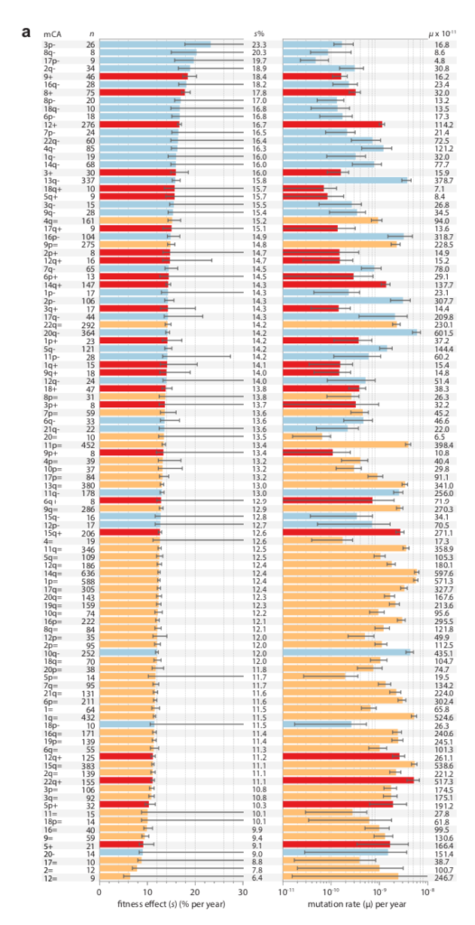
There is now a theory for this, and suggestive evidence (e.g., figure above). In “Mutation and selection induce correlations between selection coefficients and mutation rates,” Gitschlag, et al (2023) address the transformation of a joint distribution of mutation rates and selection coefficients from (1) a nominal distribution of starting possibilities, to (2) a de novo distribution of mutations (the nominal sampled by mutation rate), to (3) a fixed distribution (the de novo sampled by fitness benefit). The dual effect of mutation and selection can induce correlations, but they are not necessarily negative: they can assume any combination of signs. Yet, Gitschlag, et al (2023) argue that natural distributions will tend to have the kinds of shapes that induce negative correlations in the fixed distribution. They use simulations to illustrate these points with realistic data sets. They also show a relatively clear example in which, for the fixed distribution, selection coefficients (estimated from deep mutational scanning) are amplified for a rare mutational type, namely double-nucleotide mutations among TP53 cancer drivers. That is, the drivers that rise to clinical attention in spite of having much lower mutation rates, have greater fitness benefits that (post hoc, via conditioning) offset these lower rates.
MRE 8.13 frames this as an issue of conditioning, but that is only if one is looking backwards, making inferences from the fixed distribution. The forward problem of going from the nominal to the de novo to the fixed can be treated as an issue of what is called “size-biasing” in statistics.
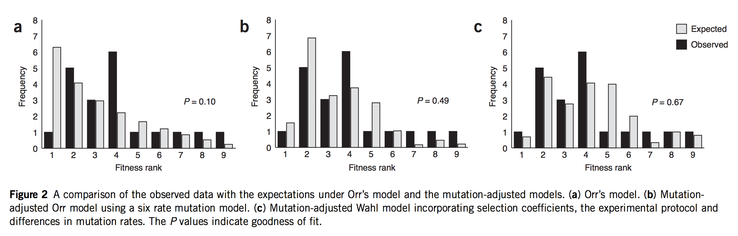
Apropos of this, I realized too late that the problem of conditioning undermines an argument from Stoltzfus and Norris (2015) that is repeated in the book (Box 9.1 or section 9.8.1). When investigating the conservative transitions hypothesis, Stoltzfus and Norris (2015) found that transitions and transversions in mutation-scanning experiments have roughly the same DFE. They also considered the DBFE (distribution of beneficial fitness effects) from laboratory adaptation experiments, which showed that beneficial transversions are slightly (not significantly) better than beneficial transitions.
At the time, this was humorously ironic: not only did we fail to find support for 50 years of lore, the data on adaptive changes actually gave the advantage to transversions.
However, we were attempting to make an inference about the nominal distribution from the fixed distribution, and therefore our inference was subject to conditioning in a way that made it unsafe: transversions that appear in the fixed distribution, in spite of their lower mutation rates, might have greater fitness benefits that (via conditioning) offset these lower rates. Thus, the pattern of more strongly beneficial transversions in the fixed distribution suggests (weakly, not significantly) a Berkson-like effect, but it does not speak against the hypothesis that the nominal DBFE is enriched for transitions (a hypothesis that, to be clear, has no direct empirical support).
Prediction about graduated effects (MRE 9.8.2)
As of 2020, all of the statistical evidence for mutation-biased adaptation in nature was based on testing for a simple excess of a mutationally favored type of change, relative to a null expectation of no bias. As MRE 9.8.2 explains, this is perfectly good evidence for mutation-biased adaptation, but not very specific as evidence for the theory of arrival biases. The theory predicts graduated effects, such that (other things being equal) a greater bias has a greater effect. In the weak-mutation regime, the effects are not just graduated, but proportional.
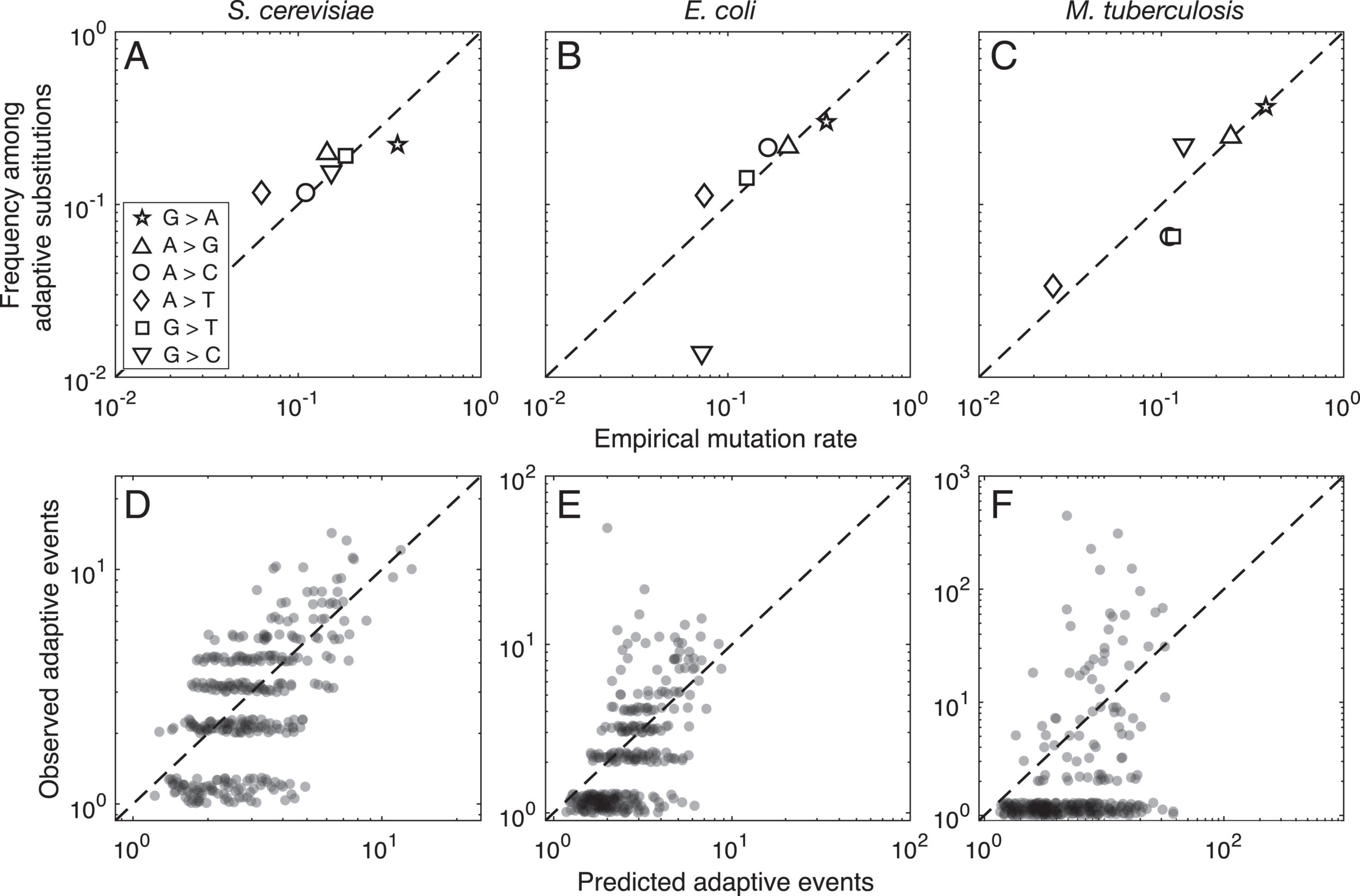
Evidence for this kind of graduated effect is now available in “Mutation bias shapes the spectrum of adaptive substitutions” by Cano, et al. (2022). The authors show a clear proportionality between the frequencies of various missense changes among adaptive substitutions, and the underlying nucleotide mutation spectrum (measured independently). They also developed a method to titrate the effect of mutation bias via a single coefficient β, defined as a coefficient of binomial regression for log(counts) vs. log(expected). Thus, one expects β to range from 0 (no effect) to 1 (proportional effect). Cano, et al. (2022) found that β is close to 1 (and significantly greater than 0) in three large data sets of adaptive changes from E. coli, yeast, and M. tuberculosis. They also split the mutation spectrum into transition bias and other effects, and found that β ~ 1 for both parts.
What this suggests generally is that each species will exhibit a spectrum of adaptive changes that reflects its distinctive mutation spectrum in a detailed quantitative way. This is precisely what the theory of arrival bias predicts, in contrast to Modern Synthesis claims (about the irrelevance of mutation rates) documented in MRE 6.4.3.
Note that the theory of arrival bias predicts graduated effects under a broad range of conditions, but only predicts β ~ 1 when the mutation supply μN is sufficiently small. Cano, et al. (2022) present simulation results showing how, as μN increases, the expected value of β drops from 1 to 0. This result applies to finite landscapes: for infinite landscapes, the effect of mutation bias does not disappear at high mutation supply (see Gomez, et al 2020).
Misleading claim: “this is expected..” (MRE 8.13)
The section on conditioning and Berkson’s paradox (see above) has the following interpretation of a result from Stoltzfus and McCandlish (2017):
When we restrict our attention to events with greater numbers of occurrences, we are biasing the sample toward higher values of μs. Thus, we expect higher values of μ, higher values of s, and a stronger negative correlation between the two. In fact, Table 9.4 shows that the transition bias tends to increase as the minimum number of occurrences is increased. This is expected, but it does not mean that the fitness effects are any less: again, we expect both higher μ and higher s, as the number of recurrences increases
The dubious part is “This is expected.” There may be a reason to expect this (I’m not entirely sure), but upon reflection, it does not relate to the paradox of conditioning that is the topic of this section, therefore the statement is misleading in context. The part that says “Thus, we expect” follows from conditioning. But the next “This is expected…” claim, if it is indeed correct, would relate to the compounding of trials. For parallelism, i.e., paths with 2 events, the effect of a bias on paths is linear and the effect of a bias on events is squared (see MRE 8.12). If we are considering only paths with 3 events or more, then we can expect an even stronger effect of mutation bias on the bias in events, because counting outcomes by events (rather than paths) is like raising the effect-size of the bias to a higher power. That is, conditioning on 3, 4 or more events per path will enrich for mutations with higher rates, whether they are transitions or transversions, but (so far as I understand) will not enrich for transition bias in the underlying paths.
Poorly phrased: “the question apparently was not asked, much less answered” (MRE 8.14)
This statement— in regard to whether 20th-century population genetics addressed the impact of a bias in introduction— sounds broader than it really is. Clearly Haldane and Fisher asked, and answered, a question about whether biases in variation could influence the course of evolution. The problem is that they didn’t ask the right question, which is about introduction biases. I’m not aware of any 20th-century work of population genetics that asks the right question. The closest is Mani and Clark, which treats the order of introductions as a stochastic variable that reduces predictability and increases variance (whereas if they had treated a bias they would have discovered that it increases predictability).
So, the claim is correct, but it is less meaningful than it sounds. Clearly the pioneers of evo-devo raised the issue of a causal link between developmental tendencies of variation and tendencies of evolution. In response, Maynard Smith, et al (1985) clearly and explicitly raised the question of how developmental biases might “cause” evolutionary trends or patterns. As recounted in MRE 8.8 and 10.2, they did not have a good answer. In general, historical evolutionary discourse includes both pre-Synthesis thinking (orthogenesis; mutational parallelisms per Vavilov or Morgan) and post-Synthesis thinking (evo-devo; molecular evolution) in which tendencies of variation are assumed or alleged to be influential, but the problem of developing a population-genetic theory for this effect was not apparently solved in the 20th century (a substantial failure of population genetics to serve the needs of evolutionary theorizing).
General issues needing clarification
Stuff that isn’t quite right, but which does not have an atomic fix.
Causal independence and statistical non-correlation
In the treatment of randomness in MRE, causal independence and statistical non-correlation are often treated as if they are the same thing. I confess that sorting this out and keeping it straight, without unduly burdening the reader, was beyond my capabilities.
The phrase “arrival bias”
The phrase “arrival of the fittest” or “arrival of the fitter” is used only twice in MRE, to refer to the thinking of others. I missed an opportunity to capitalize on “arrival bias”, a very useful and intuitive way to refer to biases in the introduction process, e.g., as in Dingle, et al (2022). Referring to the “arrival of the fittest” sounds very clever, but it combines effects of introduction and fitness in a way that is unwelcome for my purposes. Strictly speaking, arrival bias in the sense of introduction bias is an effect of the arrival of the likelier (i.e., mutationally likelier), not arrival of the fitter. One version is the “arrival of the frequent” concept of Schaper and Louis (2014), meaning a tendency for mutation to stumble upon the alternative forms that are widely distributed in genotype space.
Note that, by contrast, when Wagner (2015) refers to “the arrival of the fittest”, this is not an error of confounding mutation and fitness, but a deliberate attempt to tackle the problem of understanding how adaptive forms originate.
Quantitative evolutionary genetics
In the past, I mostly ignored QEG as irrelevant to my interests in the discrete world of molecular evolution. But in preparing to write MRE, I invested serious effort in reading the QEG literature and integrating it into my thinking about variation and causation. The biggest gap is the lack of an explanation of how and why the dispositional role of variation differs so radically in the QEG framework as compared to the kinds of models we use to illustrate arrival bias. This gap exists because the problem is unsolved.
Another issue that does not come out clearly is what, precisely, is the position of skepticism in Houle, et al. (2017), and more generally, what is the nature and extent of the neo-Darwinian refugium (or perhaps, redoubt) in the field of quantitative genetics? I incorrectly stated in MRE 5.7 that Houle, et al (2017) favor a correlational-selection-shapes-M theory, whereas their explicit position is that no known model fits their data (this position is better reflected in MRE 9.7). I am struck by the fact that the data on M:R correlation from quantitative genetics is far more rigorous and convincing than various indirect arguments of the same general form in the evo-devo literature, and yet, while the importance of “developmental bias” is often depicted as an established result in the literature of evo-devo (and EES advocacy), quantitative geneticists are clearly hesitant to conclude that the M:R correlation reflects M –> R causation, e.g., see the reference to “controversial” in the first sentence of the abstract of Houle, et al., or in Rohner and Berger (2023).
This is related to the first problem above. Variational asymmetries do not have a lot of power in the standard QEG framework: they are easily overwhelmed by selection. The quantitative geneticists understand this (and the evo-devoists perhaps do not). However, available QEG theory on effects of directional (as opposed to dimensional) bias is limited only to showing how a bias causes a slight deflection from the population optimum on a 1-peak landscape (Waxman and Peck, 2003; Zhang and Hill, 2008; Charlesworth, 2013), and lacks the kinds of multi-peak or latent-trait models that IMHO are going to show stronger effects (Xue, et al. 2015). It will be interesting to see how this plays out.
Change log
3 November 2023. Initial version with typos, updates (with a couple of figures) and Table of Contents.

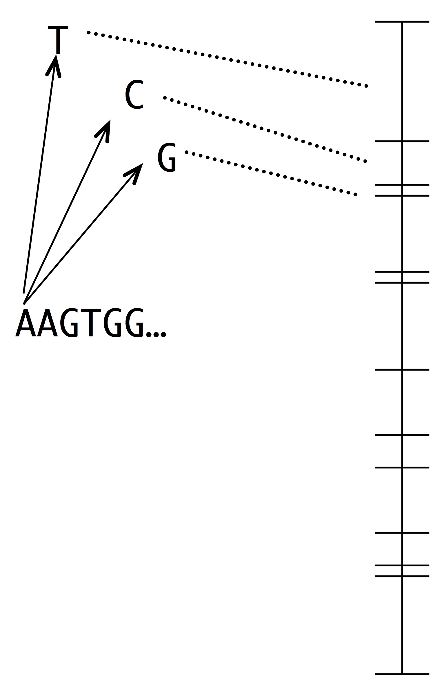
 Note two things about this idea. The first is that this is a modeling assumption, not a feature of reality. Mutations that change 2 sites at once actually occur, and presumably they sometimes contribute to evolution. The second thing to note is that we could choose to define the horizon however we want, e.g., we could include single and double changes, but not triple ones. In practice, the mutational neighbors of a sequence are always defined as the sequences that differ by just 1 residue.