Most recent update: 3 November, 2023, initial version. See the change-log at the bottom for details.
This is an ongoing list of updates and corrections to Mutation, Randomness and Evolution, including typographic errors, as well as substantive errors and updates to knowledge.
Typos and glitches
The following mistakes (given in order, by section number) might be confusing or misleading:
section 1.1 refers 3 times to a “50-fold range” of mutation rates in MacLean, et al (2010), but the actual range is 30-fold.
section 2.3. See the note about 1.1 (30-fold, not 50-fold)
in section 4.3, replace “development, growth, and hereditary” with “development, growth, and heredity”
section 4.5 describes a hypothetical experiment examining 20 mutations each for 5 species, then refers to “our small set of 20 X 10” mutations instead of “our small set of 20 X 5” mutations
section 5.7, the reference to the “ongoing commitment of evolutionary biologists to neo-Darwinism” is actually refering to the second aspect of neo-Darwinism, i.e., not adaptationism but the dichotomy of roles in which variation is subservient to selection
Fig 9.7 right panel title refers to “Frequency rate vs. fitness” instead of “Mutation rate vs. fitness”
section 9.3. See the note about 1.1 (30-fold, not 50-fold)
section A.3, the equation is mis-formatted. The left-hand side should be xi+1, not xi + 1
More recent work on topics covered in MRE
MRE was mostly completed in 2019 and only has a few citations to work published in 2020. For perspectives more up-to-date, see the following.
Ch. 8 covers the theory of arrival bias, and Ch. 9 covers evidence. Both chapters suggest generalizations that are subject to further evaluation. Most of the updates are going to involve these two chapters.
Prediction regarding self-organization (MRE 8.11)
For a long time, I’ve been arguing that one sense of “self-organization” in the work of Kauffman (1993) and others is an effect of findability that is related to the explanation for King’s codon argument, arising from biases in the introduction process (Stoltzfus, 2006, 2012). MRE 8.11 calls this “the obvious explanation for the apparent magic of Kauffman’s ‘self-organization'”, and suggests how to demonstrate this directly by implementing an artificial mutation operator that samples equally by phenotype.
This demonstration has been done— independently of my suggestions— by Dingle, et al. (2022), Phenotype Bias Determines How Natural RNA Structures Occupy the Morphospace of All Possible Shapes. The findability of intrinsically likely forms has been explored in an important series of studies from Ard Louis’s group. The earliest one, Schaper and Louis (2014), actually appeared before MRE was finished (I saw it but did not grasp the importance). More recent papers such as Dingle, et al. (2022) have made it clear that the “arrival of the frequent” or “arrival bias” in this work is a reference to biases in the introduction process that favor forms (phenotypes, folds) that are over-represented (i.e., frequent) in genotypic state-space.
Berkson’s paradox refers to associations induced by conditioning, often illustrated by an example in which a negative correlation is induced in a selected sub-population, e.g., the wikipedia page explains how a negative correlation between looks and talent could arise among celebrities if achieving celebrity status is based on a threshold of looks + talent. MRE 8.13 suggests that something like this will happen in nature, because the changes that come to our attention in spite of the disadvantage of a lower mutation rate will tend to have a larger fitness advantage, and vice versa.
Data on clonal hematopoesis lines from Watson and Blundell (2022) showing a negative correlation between growth advantage (left) and inferred mutation rate (right)
There is now a theory for this, and suggestive evidence (e.g., figure above). In “Mutation and selection induce correlations between selection coefficients and mutation rates,” Gitschlag, et al (2023) address the transformation of a joint distribution of mutation rates and selection coefficients from (1) a nominal distribution of starting possibilities, to (2) a de novo distribution of mutations (the nominal sampled by mutation rate), to (3) a fixed distribution (the de novo sampled by fitness benefit). The dual effect of mutation and selection can induce correlations, but they are not necessarily negative: they can assume any combination of signs. Yet, Gitschlag, et al (2023) argue that natural distributions will tend to have the kinds of shapes that induce negative correlations in the fixed distribution. They use simulations to illustrate these points with realistic data sets. They also show a relatively clear example in which, for the fixed distribution, selection coefficients (estimated from deep mutational scanning) are amplified for a rare mutational type, namely double-nucleotide mutations among TP53 cancer drivers. That is, the drivers that rise to clinical attention in spite of having much lower mutation rates, have greater fitness benefits that (post hoc, via conditioning) offset these lower rates.
MRE 8.13 frames this as an issue of conditioning, but that is only if one is looking backwards, making inferences from the fixed distribution. The forward problem of going from the nominal to the de novo to the fixed can be treated as an issue of what is called “size-biasing” in statistics.
Apropos of this, I realized too late that the problem of conditioning undermines an argument from Stoltzfus and Norris (2015) that is repeated in the book (Box 9.1 or section 9.8.1). When investigating the conservative transitions hypothesis, Stoltzfus and Norris (2015) found that transitions and transversions in mutation-scanning experiments have roughly the same DFE. They also considered the DBFE (distribution of beneficial fitness effects) from laboratory adaptation experiments, which showed that beneficial transversions are slightly (not significantly) better than beneficial transitions.
At the time, this was humorously ironic: not only did we fail to find support for 50 years of lore, the data on adaptive changes actually gave the advantage to transversions.
However, we were attempting to make an inference about the nominal distribution from the fixed distribution, and therefore our inference was subject to conditioning in a way that made it unsafe: transversions that appear in the fixed distribution, in spite of their lower mutation rates, might have greater fitness benefits that (via conditioning) offset these lower rates. Thus, the pattern of more strongly beneficial transversions in the fixed distribution suggests (weakly, not significantly) a Berkson-like effect, but it does not speak against the hypothesis that the nominal DBFE is enriched for transitions (a hypothesis that, to be clear, has no direct empirical support).
Prediction about graduated effects (MRE 9.8.2)
As of 2020, all of the statistical evidence for mutation-biased adaptation in nature was based on testing for a simple excess of a mutationally favored type of change, relative to a null expectation of no bias. As MRE 9.8.2 explains, this is perfectly good evidence for mutation-biased adaptation, but not very specific as evidence for the theory of arrival biases. The theory predicts graduated effects, such that (other things being equal) a greater bias has a greater effect. In the weak-mutation regime, the effects are not just graduated, but proportional.
Evidence for this kind of graduated effect is now available in “Mutation bias shapes the spectrum of adaptive substitutions” by Cano, et al. (2022). The authors show a clear proportionality between the frequencies of various missense changes among adaptive substitutions, and the underlying nucleotide mutation spectrum (measured independently). They also developed a method to titrate the effect of mutation bias via a single coefficient β, defined as a coefficient of binomial regression for log(counts) vs. log(expected). Thus, one expects β to range from 0 (no effect) to 1 (proportional effect). Cano, et al. (2022) found that β is close to 1 (and significantly greater than 0) in three large data sets of adaptive changes from E. coli, yeast, and M. tuberculosis. They also split the mutation spectrum into transition bias and other effects, and found that β ~ 1 for both parts.
What this suggests generally is that each species will exhibit a spectrum of adaptive changes that reflects its distinctive mutation spectrum in a detailed quantitative way. This is precisely what the theory of arrival bias predicts, in contrast to Modern Synthesis claims (about the irrelevance of mutation rates) documented in MRE 6.4.3.
Note that the theory of arrival bias predicts graduated effects under a broad range of conditions, but only predicts β ~ 1 when the mutation supply μN is sufficiently small. Cano, et al. (2022) present simulation results showing how, as μN increases, the expected value of β drops from 1 to 0. This result applies to finite landscapes: for infinite landscapes, the effect of mutation bias does not disappear at high mutation supply (see Gomez, et al 2020).
Misleading claim: “this is expected..” (MRE 8.13)
The section on conditioning and Berkson’s paradox (see above) has the following interpretation of a result from Stoltzfus and McCandlish (2017):
When we restrict our attention to events with greater numbers of occurrences, we are biasing the sample toward higher values of μs. Thus, we expect higher values of μ, higher values of s, and a stronger negative correlation between the two. In fact, Table 9.4 shows that the transition bias tends to increase as the minimum number of occurrences is increased. This is expected, but it does not mean that the fitness effects are any less: again, we expect both higher μ and higher s, as the number of recurrences increases
The dubious part is “This is expected.” There may be a reason to expect this (I’m not entirely sure), but upon reflection, it does not relate to the paradox of conditioning that is the topic of this section, therefore the statement is misleading in context. The part that says “Thus, we expect” follows from conditioning. But the next “This is expected…” claim, if it is indeed correct, would relate to the compounding of trials. For parallelism, i.e., paths with 2 events, the effect of a bias on paths is linear and the effect of a bias on events is squared (see MRE 8.12). If we are considering only paths with 3 events or more, then we can expect an even stronger effect of mutation bias on the bias in events, because counting outcomes by events (rather than paths) is like raising the effect-size of the bias to a higher power. That is, conditioning on 3, 4 or more events per path will enrich for mutations with higher rates, whether they are transitions or transversions, but (so far as I understand) will not enrich for transition bias in the underlying paths.
Poorly phrased: “the question apparently was not asked, much less answered” (MRE 8.14)
This statement— in regard to whether 20th-century population genetics addressed the impact of a bias in introduction— sounds broader than it really is. Clearly Haldane and Fisher asked, and answered, a question about whether biases in variation could influence the course of evolution. The problem is that they didn’t ask the right question, which is about introduction biases. I’m not aware of any 20th-century work of population genetics that asks the right question. The closest is Mani and Clark, which treats the order of introductions as a stochastic variable that reduces predictability and increases variance (whereas if they had treated a bias they would have discovered that it increases predictability).
So, the claim is correct, but it is less meaningful than it sounds. Clearly the pioneers of evo-devo raised the issue of a causal link between developmental tendencies of variation and tendencies of evolution. In response, Maynard Smith, et al (1985) clearly and explicitly raised the question of how developmental biases might “cause” evolutionary trends or patterns. As recounted in MRE 8.8 and 10.2, they did not have a good answer. In general, historical evolutionary discourse includes both pre-Synthesis thinking (orthogenesis; mutational parallelisms per Vavilov or Morgan) and post-Synthesis thinking (evo-devo; molecular evolution) in which tendencies of variation are assumed or alleged to be influential, but the problem of developing a population-genetic theory for this effect was not apparently solved in the 20th century (a substantial failure of population genetics to serve the needs of evolutionary theorizing).
General issues needing clarification
Stuff that isn’t quite right, but which does not have an atomic fix.
Causal independence and statistical non-correlation
In the treatment of randomness in MRE, causal independence and statistical non-correlation are often treated as if they are the same thing. I confess that sorting this out and keeping it straight, without unduly burdening the reader, was beyond my capabilities.
The phrase “arrival bias”
The phrase “arrival of the fittest” or “arrival of the fitter” is used only twice in MRE, to refer to the thinking of others. I missed an opportunity to capitalize on “arrival bias”, a very useful and intuitive way to refer to biases in the introduction process, e.g., as in Dingle, et al (2022). Referring to the “arrival of the fittest” sounds very clever, but it combines effects of introduction and fitness in a way that is unwelcome for my purposes. Strictly speaking, arrival bias in the sense of introduction bias is an effect of the arrival of the likelier (i.e., mutationally likelier), not arrival of the fitter. One version is the “arrival of the frequent” concept of Schaper and Louis (2014), meaning a tendency for mutation to stumble upon the alternative forms that are widely distributed in genotype space.
Note that, by contrast, when Wagner (2015) refers to “the arrival of the fittest”, this is not an error of confounding mutation and fitness, but a deliberate attempt to tackle the problem of understanding how adaptive forms originate.
Quantitative evolutionary genetics
In the past, I mostly ignored QEG as irrelevant to my interests in the discrete world of molecular evolution. But in preparing to write MRE, I invested serious effort in reading the QEG literature and integrating it into my thinking about variation and causation. The biggest gap is the lack of an explanation of how and why the dispositional role of variation differs so radically in the QEG framework as compared to the kinds of models we use to illustrate arrival bias. This gap exists because the problem is unsolved.
Another issue that does not come out clearly is what, precisely, is the position of skepticism in Houle, et al. (2017), and more generally, what is the nature and extent of the neo-Darwinian refugium (or perhaps, redoubt) in the field of quantitative genetics? I incorrectly stated in MRE 5.7 that Houle, et al (2017) favor a correlational-selection-shapes-M theory, whereas their explicit position is that no known model fits their data (this position is better reflected in MRE 9.7). I am struck by the fact that the data on M:R correlation from quantitative genetics is far more rigorous and convincing than various indirect arguments of the same general form in the evo-devo literature, and yet, while the importance of “developmental bias” is often depicted as an established result in the literature of evo-devo (and EES advocacy), quantitative geneticists are clearly hesitant to conclude that the M:R correlation reflects M –> R causation, e.g., see the reference to “controversial” in the first sentence of the abstract of Houle, et al., or in Rohner and Berger (2023).
This is related to the first problem above. Variational asymmetries do not have a lot of power in the standard QEG framework: they are easily overwhelmed by selection. The quantitative geneticists understand this (and the evo-devoists perhaps do not). However, available QEG theory on effects of directional (as opposed to dimensional) bias is limited only to showing how a bias causes a slight deflection from the population optimum on a 1-peak landscape (Waxman and Peck, 2003; Zhang and Hill, 2008; Charlesworth, 2013), and lacks the kinds of multi-peak or latent-trait models that IMHO are going to show stronger effects (Xue, et al. 2015). It will be interesting to see how this plays out.
Change log
3 November 2023. Initial version with typos, updates (with a couple of figures) and Table of Contents.
The term “mutationism” appeared in the early 20th century in regard to the views of early geneticists such as de Vries, Bateson, Punnett, and Morgan (e.g., Poulton, 1909 or McCabe 1912). These leading thinkers did not use “mutationism” to describe their own diverse views.[1] Perhaps they thought of themselves as free thinkers, not tied to any ideology or “-ism”.
In the contemporary literature, “mutationism” is most often a strawman in which evolution takes place by dramatic mutations alone, without selection (see the conceptual immune system of neo-Darwinism). This pejorative use of “mutationism” continues today in the writings of Synthesis gatekeepers such as Futuyma (2023) or Svensson (2023).
Yet the 2013 book “Mutation-driven Evolution”, by Masatoshi Nei— a pioneer of molecular evolutionary genetics who passed away in early 2023—, brought renewed attention to the idea of a broad alternative to traditional thinking focused on mutation rather than selection. Among published reviews of the book, only Wright rejects Nei’s thinking as mistaken, referring to it as “Mutationism 2.0.” Five other reviews try to explain Nei’s position sympathetically, without necessarily endorsing it. Three reviews do not mention “mutationism” (Brookfield, Galtier, Weiss). The review by Gunter Wagner entitled “The changing face of evolutionary biology”, like my review for Evo & Devo, attempts to identify a sympathetic meaning of “mutationism” appropriate for Nei’s distinctive project, focusing on the importance of mutations in evolution.
One might be tempted to avoid the term “mutationism” (along with “saltationism” and “orthogenesis”) on the grounds of being toxic. To use this term is to risk ridicule and invite misunderstanding. Why do that, when one’s goal is to communicate with readers? I avoided these terms myself for many years, on precisely these grounds. However, eventually I decided not to acquiesce to rhetorical tactics designed to browbeat dissenters using strawman arguments. As we say here in the US, that would be letting the terrorists win. Promoting good intellectual hygiene in our field means calling out fallacies, and addressing alternative views fairly and rigorously, without rhetorical trickery. [2]
If “selectionism” is allowable to designate a focus on selection, without denying a role for mutations in evolution, then “mutationism” is allowable to designate a focus on mutation that does not deny selection.
If there are distinctive features of the views of Nei and the early geneticists, nothing prevents us from using “mutationism” to denote those features. If “selectionism” is allowable to designate a focus on selection, without denying a role for mutations in evolution, then “mutationism” is allowable to designate a focus on mutation that does not deny selection. In my own thinking, I tend to associate “mutationism” with a non-exclusive explanatory position, with the lucky-mutant conception of evolutionary dynamics (see the shift to mutationism is documented in our language), or with a school of thought.
TLDR
Possible meaning of mutationism
Type of meaning
evolution happens by dramatic mutations alone, without selection
Strawman from Synthesis tribal mythology, employed by gatekeepers to police orthodoxy
identifying distinctive mutational-developmental changes is a uniquely powerful way to explain the evolution of form
Explanatory position on what kinds of causal attributions are meaningful, key to evo-devo
reconstructing mutational changes provides uniquely reliable knowledge of past evolution
Methodological position on which causes are most accessible to scientific methods, also key in evo-devo
the timing and character of events of mutation determine the timing and character of evolutionary change
Empirical position on evolutionary dynamics, e.g., in applications of origin-fixation models
diverse evolutionary phenomena arise from combining mutation and genetics
Loosely defined school of thought associated with Bateson, Punnett and Morgan
a preliminary and imperfect expression of (for instance) a future paradigm of dual causation
Transition state mainly of historical interest
The Mutationism Story in Synthesis tribal mythology
In the mainstream literature of evolutionary biology, history is told in a way that makes things turn out right for the Modern Synthesis, e.g., there is literally an “eclipse of Darwinism”— a period of darkness and strife— that ends when the Modern Synthesis solves the problem of evolution. This self-serving view of history is called “Synthesis Historiography” or SH by professional historians (Amundson, 2005). In SH, critics of neo-Darwinism behave irrationally and hold views with obvious flaws, while Darwin’s followers use reason and evidence to establish important truths.
The stories in SH function as a tribal mythology, i.e., scientists who identify culturally with the “Synthesis” tell these stories to each other to affirm their identity, which is based on a shared belief in their fundamental rightness about evolution, and the wrongness of historic opponents. For instance, in the Mutationism Story, the early geneticists are too stupid to understand populations, gradual change, or selection, which they reject, believing instead that evolution happens by dramatic mutations alone, without selection. The problem is solved when Fisher sees what the mutationists are too foolish to see: there is no conflict between gradualism, selection, and genetics. Versions of this fable are given in this blog (e.g., Dawkins 1987, p. 305 of The Blind Watchmaker; Cronin 1991, p. 47 of The Ant and the Peacock; Ayala and Fitch 1997; Futuyma, 2017; Segerstråle 2002, Oxford Encyclopedia of Evolution 2, pp. 807 to 810; Charlesworth and Charlesworth 2009). Here is Dawkins’s version:
“It is hard for us to comprehend but, in the early years of this century when the phenomenon of mutation was first named, it was regarded not as a necessary part of Darwinian theory but as an alternative theory of evolution! There was a school of geneticists called the mutationists, which included such famous names as Hugo de Vries and William Bateson among the early rediscoverers of Mendel’s principles of heredity, Wilhelm Johannsen the inventor of the word gene, and Thomas Hunt Morgan the father of the chromosome theory of heredity. . . Mendelian genetics was thought of, not as the central plank of Darwinism that it is today, but as antithetical to Darwinism. . . It is extremely hard for the modern mind to respond to this idea with anything but mirth”
Dawkins, 1987, p. 305
Actual history contradicts the Mutationism Story. In reality, immediately upon the discovery of genetics in 1900, early geneticists began to assemble the pieces of a Mendelian view of evolution by mutation, inheritance, and differential survival (Stoltzfus and Cable 2014). The multiple-factor theory was immediately suggested by Bateson and others. Here Bateson and Saunders (1902) give a precise verbal rendition of the Hardy-Weinberg paradigm, the first rigorous paradigm of population thinking:
“It will be of great interest to study the statistics of such a population in nature. If the degree of dominance can be experimentally determined, or the heterozygote recognised, and we can suppose that all forms mate together with equal freedom and fertility, and that there is no natural selection in respect of the allelomorphs, it should be possible to predict the proportions of the several components of the population with some accuracy. Conversely, departures from the calculated result would then throw no little light on the influence of disturbing factors, selection, and the like.”
Bateson and Saunders, 1902, p. 130
Thomas Hunt Morgan won a Nobel prize in genetics. His tendency to refer to “survival” of “definite variations” and to avoid “natural selection” reflects, not a rejection of what we call “selection” today, nor some kind of mental block, but a belief that shifting the goal-posts to avoid accountability is bad for science. For Morgan, the term “natural selection” must be reserved for Darwin’s non-Mendelian theory based on the blending of environmentally stimulated fluctuations (“indefinite variability”), a theory correctly rejected by the scientific community when it was experimentally refuted by Johannsen. Morgan called out the problem of goal-post-shifting when he wrote that “Modern zoologists who claim that the Darwinian theory is sufficiently broad to include the idea of the survival of definite variations seem inclined to forget that Darwin examined this possibility and rejected it.” (Morgan, 1904).
The early geneticists did not reject what we would call “selection” today, e.g., Morgan (1916), in his closing summary, writes that “Evolution has taken place by the incorporation into the race of those mutations that are beneficial to the life and reproduction of the organism” (p. 194). Bateson, Punnett, de Vries and Johannsen were the other early geneticists most well known for their views on evolution. Johannsen and de Vries both carried out successful selection experiments. de Vries begins his major 1905 English treatise by writing that …
“Darwin discovered the great principle which rules the evolution of organisms. It is the principle of natural selection. It is the sifting out of all organisms of minor worth through the struggle for life. It is only a sieve, and not a force of nature” (p. 6)
In Materials for the Study of Variation, Bateson (1894) refers to natural selection as “obviously” a “true cause” (p. 5). Punnett (1905) explains that mutations are heritable while environmental fluctuations are not, concluding that “Evolution takes place through the action of selection on these mutations” (p. 53).
Morgan called out the problem of goal-post-shifting when he wrote that “Modern zoologists who claim that the Darwinian theory is sufficiently broad to include the idea of the survival of definite variations seem inclined to forget that Darwin examined this possibility and rejected it.” (Morgan, 1904).
The views of these influential scientists, and their contributions to evolutionary thinking, were not secrets: they were published, cited and discussed. Bateson, Punnett, Morgan and de Vries all were awarded the Royal Society Darwin medal in the period from 1900 to 1930. That is, the Mutationism Story is not just a wildly distorted version of history: it is a wildly distorted version of history contradicted by sources that are readily accessible to any serious scholar. The ongoing success of this kind of mythology is a testament to the power of propaganda and to the insularity of the Synthesis tribal culture (again, see the conceptual immune system).
Explanatory or methodological mutationism
Explanatory and methodological versions of mutationism are useful to contemplate, by comparison to the flavors of adaptationism identified by Godfrey Smith (2001):
Empirical adaptationism is ontological, based on a belief about how the world actually is: living things are pervasively adapted, down to the finest detail, and therefore, we will see adaptation everywhere we look because adaptation is in fact everywhere we look, and the explanation for traits will inevitably be functional because traits are in fact inevitably functional.
Methodological adaptationism holds that, even though adaptation might not be pervasive, it is the thing we are uniquely equipped to study using the methods of science. This view tends to travel together with the ideology that evolution is a combination of selection and “chance”, with the latter being hard to study systematically.
Explanatory adaptationism is the view that, although selection might not be everything, and although we might be able to study other kinds of causes in evolution, a focus on selection and adaptation is justified because adaptation is the distinctive problem in evolution, and selection is the necessary principle behind adaptation.
Analogously, we can imagine empirical, explanatory, and methodological versions of mutationism. The lucky mutant view mentioned below is one possible ontological or empirical flavor of mutationism. In methodological mutationism, which is clearly a research program in evo-devo, we focus on identifying the mutational-developmental changes involved in evolution on the grounds that this is a distinctively reliable and productive way to study evolution. In explanatory mutationism, our focus is on identifying the detailed mutational-developmental changes underlying changes in form, because explaining changes in form over time is the distinctive challenge of evolutionary biology.
Clearly we can study the evolution of form from a structuralist viewpoint as a series of transformations based on genetic encodings and the intrinsic self-organizing properties of material systems, but we also can study the evolution of form from an adaptationist perspective.
Bateson’s early work exemplifies methodological mutationism: he believed that, in order to understand how evolution happens, the first step was to study variations. Accordingly, his Materials for the Study of Variation is a catalog of 886 numbered cases of discontinuous variations. Bateson planned a second volume on continuous variation but subsequent work on quantitative trait distributions made this unnecessary.
Bateson’s approach was observational, but today we see various experimentallyoriented mutationist projects in evolutionary biology:
attempts to reconstruct mutational changes involved in key changes in development, in the context of evo-devo
systematic measurements of M in quantitative genetics, e.g., Houle, et al (2017)
reconstructing ancestral protein molecules and their mutants in order to reconstruct the path of history and test hypotheses (from biochemically-oriented molecular evolutionists, e.g., Dean, Weinreich, Thornton, et al)
the recent focus on using deep sequencing methods to characterize the mutation spectrum in quantitative detail in a variety of organisms, and in the context of cancer biogenesis
Note that these projects are generally situated in paradigms that are not focused solely on mutation, but also reflect functionalist concerns. This is clearly true of evo-devo, for instance, as the analysis of Novick (2023) makes clear. The evo-devoists are not merely concerned with understanding why certain types of transformations are mutationally and developmentally likely, they are also concerned with selection and function. The same is obviously true of the line of work from Thornton and colleagues, which combines the reconstruction of mutants with functional assays and even selection experiments. In the study of cancer drivers and clonal haematopoesis mutants, contemporary research on mutation spectra, mutation rates, and repair mutants is premised on the understanding that clinical prevalence reflects both the rate of mutational origin and the selection intensity (figure; see Cannataro, et al. 2019; Watson and Blundell, 2022).
Estimates of selection intensity (left) and rate of mutation (right) for clonal haematopoesis lineages from Watson and Blundell (2022). Yes, there is a negative correlation. Why values of s and u might be negatively correlated (in the distribution after mutation and selection) is a question addressed in Gitschlag, et al (2023).
If we look at methodological mutationism as an extreme or exclusive position, it is difficult to separate from an extreme form of skepticism about selection that seems unwarranted today, when we can test hypotheses of selection in rigorous ways and assign some non-negligible proportion of the variance in outcomes to selection. Apropos, Nei (2013) does not reject selection as a causal principle in evolution, yet in practice, he seems to reject every attempt to attribute something concrete to positive selection. His approach recalls the attitude of Bateson, who (a century earlier) disparaged adaptationist story-telling by appealing to Voltaire’s Dr. Pangloss, a trope made famous in the “Panglossian paradigm” of Gould and Lewontin (1979). A scientist in Bateson’s time might find it easy to dismiss the vast majority of claims about selection as armchair speculation, not science. Punnett was so deeply skeptical of adaptive explanations that he rejected adaptive mimicry as an explanation for apparently mimetic morphs in butterflies!
Likewise, it’s hard to think of explanatory mutationism as an exclusive position. Clearly we can study the evolution of form from a structuralist viewpoint as a series of transformations based on genetic encodings and the intrinsic self-organizing properties of material systems, but we also can study the evolution of form from an adaptationist perspective.
So, rather than supposing that mutationism is uniquely explanatory for evolution in general, perhaps we can suppose instead that it is distinctively explanatory in some limited but important context. What is the limited but important context in which selective explanations are the least informative or trustworthy, and in which mutational explanations have more power to explain what we wish to understand? I think the best answer here is that there are some aspects of deep divergence, such as the formation of new body plans, major taxa, or key innovations, in which the power of selective explanations is at its lowest—because there are too many degrees of freedom— and the power of mutational explanations are at their highest, e.g., when key innovations can be associated with specific changes in developmental genetics, against a background of conserved features that do not change.
Mendelo-mutationism as a school of thought
The “school of thought” version of Mendelian mutationism is not a unified theory, but a loose collection of beliefs and ideas, overlapping substantially with how the “Modern Synthesis” is construed mistakenly today as a loose collection of beliefs consistent with genetics and selection (see this blog or Stoltzfus and Cable, 2014 for a review).
The early geneticists were the first scientists to accept particulate inheritance and mutation as the foundation of their understanding of evolution, in the sense that they viewed with suspicion any idea that could not be reconciled with particulate inheritance and mutation. Adopting genetics as the foundation for evolutionary reasoning sounds very familiar today, but in 1909 this was a disruptive view that seems to have pissed off evolutionists who were not geneticists, i.e., most of them. Imagine these upstarts telling leading evolutionary thinkers— paleontologists, systematics, embryologists— that the foundation for all thinking in evolution must be particulate inheritance and mutation, new discoveries only understood by a small group of scientists!
As noted above, Bateson and Saunders (1902) clearly articulated the research program of looking for deviations from Hardy-Weinberg expectations as a way of detecting causes other than inheritance.
In the same 1902 paper, they explain what became known as “the multiple factor theory” in which a smooth distribution of trait-values reflects, not blending inheritance and fluctuation, but the joint effect of Mendelian variation at many loci, combined with environmental noise.
Adopting genetics as the foundation for evolutionary reasoning sounds very familiar today, but in 1909 this was a disruptive view that seems to have pissed off evolutionists who were not geneticists, i.e., most of them.
But of course they also considered non-gradual changes via distinctive mutations, i.e., saltations. To the extent that non-gradual changes reflecting distinctive mutations are important in evolution, understanding evolution requires knowing how and when these distinctive mutations arise, based on relevant theories and systematic data. This is why Bateson (1894) catalogued distinctive variations as a way of understanding evolution. Morgan later made a systematic search for mutations in fruit-flies. It was Morgan who first clearly depicted evolution as a series of mutations that are accepted by virtue of being beneficial to the survival of the species. He articulated the concept of a probability of fixation in 1916, distinguishing the case of beneficial, neutral and deleterious mutations (the mathematical problem was later solved partially by Haldane, 1927 and more thoroughly by Kimura, 1962).
Interestingly, it was also Morgan (1909) who first suggested the randomness of mutation as a kind of metaphysical gambit, a working assumption that, so long as the origins of mutations remain a mystery, we will treat them as random and not entertain any ideas in which they have special properties.
Whether definite variations are by chance useful, or whether they are purposeful are the contrasting views of modern speculation. The philosophic zoologist of to-day has made his choice. He has chosen undirected variations as furnishing the materials for natural selection. It gives him a working hypothesis that calls in no unknown agencies; it accords with what he observes in nature; it promises the largest rewards. He does not deny, if he is cautious, the possibility that there may be a purposefulness in the sense that organisms may respond adaptively at times to external conditions; for the very basis of his theory rests on the assumption that such variations do occur. But he is inclined to question the assumption that adaptive variations arise because of their adaptiveness. In his experience he finds little evidence for this belief, and he finds much that is opposed to it. He can foresee that to admit it for that all important group of facts, where adjustments arise through the adaptation of individuals to each other—of host to parasite, of hunter to hunted—will land him in a mire of unverifiable speculation.
Note again the stark contrast between the facts of history and the stories used in Synthesis gatekeeping, in which an association of “mutationism” with directed mutation has been fabricated repeatedly in the attempt to discredit both (Gardner, 2013; Svensson, 2023).
However, Morgan frequently noted that mutations happen at different rates. He and Punnett both believed that this was important for evolution, and might play a role in parallel evolution, citing cases like albino or melanic forms. Under a neo-Darwinian view, melanic forms are expected to emerge gradually, like the all-black rats in Castle’s experiments, from the gradual accumulation of many small differences; and the repeated appearance of melanism in different taxa would indicate that it is some kind of adaptive optimum. For the mutationists, the repeated occurrence of melanic forms suggested that such forms were readily mutationally accessible.
Vavilov (1922) took this idea of parallel evolution by parallel variations to extreme lengths. From his extensive observations of plants, especially crop species, he developed a theory that each major group of organisms has a set of characteristic variants that eventually manifest as distinct species, e.g., if family F has a tendency to produce long-eared forms, this tendency would manifest in genera G1, G2, … each having both long-eared and short-eared species within the genus. He also proposed a kind of mimicry— now called Vavilovian mimicry— that turns out to be quite important among domesticated crop species. In Vavilovian mimicry, the model is a cultivated species actively harvested and propagated by humans, and the mimic starts out as a weed that is eventually propagated by humans by virtue of mimicking the model in terms of the time of maturation, and similar responses to threshing and winnowing techniques. For instance, rye and oats are believed to be Vavilovian mimics that emerged in the context of wheat cultivation (see the wikipedia article on Vavilovian mimicry).
With regard to species and speciation, the early geneticists tended to believe that reproductive incompatibilities were “the true criterion of what constitutes a species” (Punnett, 1911, p. 151). With the Modern Synthesis, this “biological species concept” became the prevailing view (Mallet 2013). They allowed for different kinds of speciation, including speciation by non-Mendelian mutations like de Vriesian macromutations, but also by the accumulation of what we now call “Bateson-Dobzhansky-Muller” incompatibilities.
To summarize, the early geneticists opened up and explored a new field, considering a wide range of possibilities (excluding only Lamarckism) and contributing a number of key concepts to evolutionary genetics. Few people know of their accomplishments today because, in Synthesis Historiography, scientific progress only comes from people with the right Darwinian lineage, and not from critics of neo-Darwinism, who are treated as aliens or un-persons. For instance, in Synthesis Historiography, the credit for rejecting 19th-century views of heredity and introducing modern notions of hard inheritance is awarded, not to the geneticists responsible for this innovation, but to 19th-century physiologist and infamous mouse-torturer August Weismann. The Oxford Encyclopedia of Evolution does not have biographic entries for Bateson, de Vries, Punnett, or other early geneticists except for the entry on Morgan, which says nothing of his views of evolution, although he wrote 4 books on the topic. For a graphical example of how the early geneticists are treated as un-persons in Synthesis Historiography, read this.
Lucky mutant (sushi conveyor) dynamics
The lucky mutant version of mutationism is a focus on the regime of population genetics in which origination events are important, so that the timing and character of evolutionary change depend on the timing and character of events of mutation that introduce new alleles (or phenotypes). This is sometimes called “mutation-driven” or “mutation-limited” evolution. For me, “mutation-driven” evokes evolution by mutation pressure, so I don’t like the term, but I feel obliged to use it occasionally because this is what some readers recognize. The problem with “mutation-limited” is that, for the vast majority of readers, it suggests some kind of limit to the outcomes that selection can access, whereas for theoreticians this is a statement about dynamics.[3]
As a technical description of dynamics, “mutation-limited” behavior could mean either (1) behavior responsive to changes in u or (2) the limiting behavior as u approaches 0, which is origin-fixation dynamics. When people like Dawkins (2007) invoke the idea that “evolution is not mutation-limited” as a way of discounting a focus on mutation, this only makes sense if it means that evolutionary behavior is not responsive to changes in u, which is what Dobzhansky and others stated explicitly, i.e., they said that changing the rate of mutation would not change the rate of evolution due to the buffering capacity of the gene-pool.
In other words, the most direct label for mutation-responsive dynamics would be “mutation-responsive dynamics” rather than “mutation-limited” or “mutation-driven” dynamics. I have also referred to the “sushi-conveyor” regime of population genetics, as distinct from the “buffet” regime.
Defining “mutationism” as a position on population genetics is not the most historically justifiable way to interpret the views of the early geneticists, because they were not very explicit about population genetics. However, it is how we might choose to see mutationism in retrospective contrast to the neo-Darwinian view of the Modern Synthesis. Darwin’s followers, in their dialectical encounter with the early geneticists, were most concerned to defend the power and creativity of selection, to defend gradualism, and to reject a lucky mutant view of dynamics. They did this by invoking the “buffet” regime of population genetics, in which evolution takes place by shifting the frequencies of alleles present in an abundant gene pool.
The sushi conveyor: We iteratively make a yes-or-no choice on the chef’s latest creation as it passes by on a moving conveyor. A bias in the rate of appearance directly biases the outcome.
Consider again the example of melanic or albino morphs. The repeated occurrence of melanic morphs in related species might suggest to us the possibility of a common mutation to blackness that has occurred repeatedly. Under neo-Darwinism, by contrast, this would only happen by the accumulation of many small effects, i.e., in the same way that all-black rats emerged in the Castle experiment from the accumulation of many small variations. Note that the historic reception of Castle’s experiment illustrated the breadth of mutationist thinking: in a famous dispute with Castle and colleagues, members of Morgan’s group insisted that the gradual emergence of all black and all white rats was entirely consistent with incremental frequency shifts of small-effect alleles under the Mendelian multiple-factor theory, and did not require blending or transformation of hereditary factors, as Castle (under the influence of Darwin’s thinking) had argued.
If “mutationism” means the lucky-mutant view of sushi-conveyor dynamics, then we have seen a broad resurgence of mutationism in evolutionary biology, starting with the molecular evolutionists in the 1960s. See The shift to mutationism is documented in our language.
A transition to …
Finally we can think of mutationism not as a resting point or destination, but as an unstable transition-state on the path to something else. The most productive line of thought, perhaps, is that it points the way toward a paradigm of dual causation that combines functionalism and structuralism, with a major goal of partitioning variance in outcomes to variational and selective causes. A clear and direct recognition of dual causation is evident in statements of Vavilov (1922), e.g.,
“the role of natural selection in this case is quite clear. Man unconsciously, year after year, by his sorting machines, separated varieties of vetches similar to lentils in size and form of seeds, and ripening simultaneously with lentils. The same varieties certainly existed long before selection itself, and the appearance of their series [i.e., combinations], irrespective of any selection, was in accordance with the laws of variation.” (p. 85)
Here Vavilov combines two different kinds of dispositions in one theory, such that each disposition reflects a set of distinct causal processes that are invoked directly in historical explanations. Darwin’s followers would look at the same case and say that variation merely supplies raw material that selection shapes into adaptations, invoking two kinds of causal processes, only one of which is dispositional.
One sees a notion of dual causation expressed very abstractly by Vrba and Eldredge (1984), in their enhanced description of evo-devo thinking:
“Developmental biologists variously stress: (1) how indirect any genetic control is during certain stages of epigenesis; (2) that the system determines by downward causation which genomic constituents are stored in unexpressed form versus those which are expressed in the phenoytpe; (3) that bias in the introduction of phenotypic variation may be more important to directional phenotypic evolution than sorting by selection. This is in contrast to the synthesis, which stresses more or less direct upward causation from random mutations to phenotypic variants, with selection among the latter as the prime determinant of directional evolution.”
Instead of casting evolution as shifting gene frequencies, we can depict it more broadly as a process of the introduction and reproductive sorting of variation in a hierarchy of reproducing entities.[4] To the extent that evolution has any predictable tendencies, they reflect biases in introduction and biases in sorting. This is not simply a re-statement of the position of Vavilov or of Vrba and Eldredge, which is not based on any technical understanding of bias in the introduction of variation as a population-genetic mechanism.
However, the reason for the resurgence of interest in quasi-mutationist thinking— as an attempt to get beyond neo-Darwinism— is that selection does not actually govern evolution in the way that neo-Darwinism supposes. It is a directional factor, but not the directional factor.
The classical functionalist position of neo-Darwinism and the Modern Synthesis focuses on biases in reproductive sorting (i.e., selection) as the cause of everything interesting. The success of this research program is proof that effects of biases in reproductive sorting are profoundly important in evolution. However, the reason for the resurgence of interest in quasi-mutationist thinking— as an attempt to get beyond neo-Darwinism— is that selection does not actually govern evolution in the way that neo-Darwinism supposes. Selection is a directional factor, but not the directional factor. We can also pursue a research program based on the role of generative biases in evolution and, even more broadly, a research program that focuses on both biases in the introduction of variation and biases in the reproduction of variation, with the goal of quantifying their relative influence on the predictability of evolution.
References
Bateson W. 1894. Materials for the Study of Variation, Treated with Especial Regard to Discontinuity in the Origin of Species. London: Macmillan.
Bateson W, Saunders ER. 1902. Experimental Studies in the Physiology of Heredity. In. Reports to the Evolution Committee: Royal Society.
Davenport CB. 1909. Mutation. In. Fifty Years of Darwinism: Modern Aspects of Evolution. New York: Henry Holt and Company. p. 160-181.
Dawkins R. 2007. Review: The Edge of Evolution. In. International Herald Tribune. Paris. p. 2.
de Vries H. 1905. Species and Varieties: Their Origin by Mutation. Chicago: The Open Court Publishing Company.
Futuyma DJ. 2017. Evolutionary biology today and the call for an extended synthesis. Interface Focus 7:20160145.
Godfrey-Smith P. 2001. Three Kinds of Adaptationism. In: Orzack SH, Sober E, editors. Adaptationism and Optimality. Cambridge: Cambridge University Press. p. 335-357.
Gould SJ, Lewontin RC. (classic; CNE theory co-authors). 1979. The spandrels of San Marco and the Panglossian paradigm: a critique of the adaptationist program. Proc. Royal Soc. London B 205:581-598.
McCabe J. 1912. The Story of Evolution.
Morgan TH. 1904. The Origin of Species through Selection Contrasted with their Origin through the Appearance of Definite Variations. Popular Science Monthly:54-65.
Morgan TH. 1909. For Darwin. Popular Science Monthly 74:367-380.
Morgan TH. 1916. A Critique of the Theory of Evolution. Princeton, NJ: Princeton University Press.
Nei M. 2013. Mutation-Driven Evolution: Oxford University Press.
Novick R. 2023. Structure and Function. In. Cambridge: Cambridge University Press.
Poulton EB. 1909. Fifty Years of Darwinism. In. Fifty Years of Darwinism: Modern Aspects of Evolution. New York: Henry Holt and Company. p. 8-56.
Punnett RC. 1905. Mendelism. London: MacMillan and Bowes.
Punnett RC. 1911. Mendelism: MacMillan.
Segerstråle U. 2002. Neo-Darwinism. In: Pagel M, editor. Encyclopedia of Evolution. New York: Oxford University Press. p. 807-810.
Stamhuis IH. 2015. Why the Rediscoverer Ended up on the Sidelines: Hugo De Vries’s Theory of Inheritance and the Mendelian Laws. Science & Education 24:29-49.
Stoltzfus A, Cable K. 2014. Mendelian-Mutationism: The Forgotten Evolutionary Synthesis. J Hist Biol 47:501-546.
Svensson EI. 2023. The structure of evolutionary theory: beyond Neo-Darwinism, Neo-Lamarckism and biased historical narratives about the Modern Synthesis. In: Dickins TE, Dickins JA, editors. Evolutionary biology: contemporary and historical reflections upon core theory. Cham, Switzerland: Springer Nature.
Vavilov NI. 1922. The Law of Homologous Series in Variation. J. Heredity 12:47-89.
Vrba ES, Eldredge N. (benchmark; co-authors). 1984. Individuals, hierarchies and processes: towards a more complete evolutionary theory. Paleobiology 10:146-171.
Notes
[1] The term “early geneticist” typically means scientists working on mutation and Mendelian inheritance in the first decade of the 20th century (thus Goldschmidt is not considered an early geneticist). The most influential ones were clearly Johannsen, de Vries, Bateson, Punnett, and Morgan. My claim that leading early geneticists did not use the term “mutationism” for their own views is based on published works of Bateson, Punnett, Morgan and de Vries. I’m not going to say they never used it, but I haven’t found a case. I found one instance where Davenport (1909) refers to the view of the “the mutationist”. De Vries literally proposed a MutationsTheorie so it is natural to call him a mutationist. But de Vries’s thinking was extremely complex and mainly non-Mendelian, and the other early geneticists developed their own views, not relying on de Vries’s thinking (for explanation, see Stoltzfus and Cable, 2014).
[2] I’m saying this as an established researcher who is not trying to get a job or tenure, or to curry favor with decision-makers. If you are a junior person, calling out the strawman arguments and shoddy historical scholarship used by influential gatekeepers poses risks to your career, and you should weigh those risks carefully. It’s perfectly all right to leave this fight to others who are not as vulnerable. We all have to pick our battles, and mine are not the same as yours.
[3] For instance, consider evolution under mutation bias on a smooth landscape with one peak. Ultimately the system goes to the peak: mutation places no limits in this sense. However, the rate and trajectory of the approach to the peak will reflect the rate and bias of mutations. So, the dynamics are mutation-responsive but the ultimate outcome and the ultimate level of fitness or adaptation is not limited by mutation. If multiple peaks or destinations are possible, then biases in introduction may be influential. Calling this mutation-limited evolution would just confuse people; saying that it isn’t mutation-limited also would give the wrong impression.
[4] Technically the list should be something more like “introduction, hereditary transmission and reproductive sorting” with biases possible in each process. Biased gene conversion is a transmission bias. So is meiotic drive. Effects of mutational hazard in the thinking of Lynch can be understood as biases in transmission, i.e., longer sequences have lower transmission due to mutational damage (mutational hazard is not an effect of introduction; although it is possible to cast it as a form of selection, that is weird IMHO).
This post started out as a wonky rant about why a particular high-profile study of laboratory adaptation was mis-framed as though it were a validation of the mutational landscape model of Orr and Gillespie (see Orr, 2003), when in fact the specific innovations of that theory were either rejected, or not tested critically. As I continued ranting, I realized that there was quite a bit to say that is educational, and I contemplated that the reason for the original mis-framing is that this is an unfamiliar area, such that even the experts are confused— which means that there is a value to explaining things.
The crux of the matter is that the Gillespie-Orr “mutational landscape” model has some innovations, but also draws on other concepts and older work. We’ll start with these older foundations.
In origin-fixation models, evolution is seen as a simple 2-step process of the introduction of a new allele, and its subsequent fixation (image). The rate of change is then characterized as a product of 2 factors, the rate of mutational origin (introduction) of new alleles of a particular type, and the probability that a new allele of that type will reach fixation. Under some general assumptions, this product is equal to the rate of an origin-fixation process when it reaches steady state.
Probably the most famous origin-fixation model is K = 4Nus, which uses 2s (Haldane, 1927) for the probability of fixation of a beneficial allele, and 2Nu (diploids) for the rate of mutational origin. Thus K = 4Nus is the expected rate of changes when we are considering types of beneficial alleles that arise by mutation at rate u, and have a selective advantage s. But we can adapt origin-fixation dynamics to other cases, including neutral and deleterious changes. If we were applying origin-fixation dynamics to meiotic bursts, or to phage bursts, in which the same mutational event gives rise immediately to multiple copies (prior to selection), we would use a probability of fixation that takes this multiplicity into account.
In passing, note that origin-fixation models appeared in 1969, and we haven’t always viewed evolution this way. The architects of the Modern Synthesis rejected this view— and if you don’t believe that, read The Shift to Mutationism is Documented in Our Language or The Buffet and the Sushi Conveyor. They saw evolution as more of an ongoing process of “shifting gene frequencies” in a super-abundant “gene pool” (image). Mutation merely supplies variation to the “gene pool”, which is kept full of variation. The contribution of mutation is trivial. The available variation is constantly mixed up by recombination, represented by the egg-beaters in the figure. When the environment changes, selection results in a new distribution of allele frequencies, and that’s “evolution”— shifting gene frequencies to a new optimum in response to a change in conditions.
This is probably too geeky to mention, but from a theoretical perspective, an origin-fixation model might mean 2 different things. It might be an aggregate rate of change across many sites, or the rate applied to a sequence of changes at a single locus. The mathematical derivation, the underlying assumptions, and the legitimate uses are different under these two conditions, as pointed out by McCandlish and Stoltzfus. The early models of King, et al were aggregate-rate models, while Gillespie, (1983) was the first to derive a sequential-fixations model.
Second, the mutational landscape model draws on Maynard Smith’s (1970) concept of evolution as discrete stepwise movement in a discrete “sequence space”. More specifically, it draws on the rarely articulated locality assumption by which we say that a step is limited to mutational “neighbors” of a sequence that differ by one simple mutation, rather than the entire universe of sequences. The justification for this assumption is that double-mutants, for instance, will arise in proportion to the square of the mutation rate, which is a very small number, so that we can ignore them. Instead, we can think of the evolutionary process as accessing only a local part of the universe of sequences, which shifts with each step it takes. In order for adaptive evolution to happen, there must be fitter genotypes in the neighborhood.
This is an important concept, and we ought to have a name for it. I call it the “evolutionary horizon”, because we can’t see beyond the horizon, and the horizon changes as we move. Note two things about this idea. The first is that this is a modeling assumption, not a feature of reality. Mutations that change 2 sites at once actually occur, and presumably they sometimes contribute to evolution. The second thing to note is that we could choose to define the horizon however we want, e.g., we could include single and double changes, but not triple ones. In practice, the mutational neighbors of a sequence are always defined as the sequences that differ by just 1 residue.
Putting these 2 pieces together, we can formulate a model of stepwise evolution with predictable dynamics.
Making this into a simulation of evolution is easy using the kind of number line shown at left. Each segment represents a possible mutation-fixation event from the starting sequence. For instance, we can change the “A” nucleotide that begins the sequence to “T”, “C” or “G”. The length of each segment is proportional to the origin-fixation probability for that change (where the probability is computed from the instantaneous rate). To pick the next step in evolution, we simply pick a random point on the number line. Then, we have to update the horizon— recompute the numberline with the new set of 1-mutant neighbors.
Where do we get the actual values for mutation and fixation? One way to do it is by drawing from some random distribution. I did this in a 2006 simulation study. I wasn’t doing anything special. It seemed very obvious at the time.
(Table 1 from Rokyta, et al)
Surprisingly, researchers almost never measure actual mutation and selection values for relevant mutants. One exception is the important study by Rokyta, et al (2005), who repeatedly carried out 1-step adaptation using bacteriophage phiX174. The selection coefficients for each of the 11 beneficial changes observed in replicate experiments are shown in the rightmost column, with the mutants ranked from highest to lowest selection coefficient. Notice that the genotype that recurred most often (see the “Number” column) was not the alternative genotype with the highest fitness, but the 4th-most-fit alternative, which happened to be favored by a considerable bias in mutation. Rokyta, et al didn’t actually measure specific rates for each mutation, but simply estimated average rates for different classes of nucleotide mutation based on an evolutionary model.
Then Rokyta, et al. developed a model of origin-fixation dynamics using the estimated mutation rates, the measured selection coefficients, and a term for the probability of fixation customized to account for the way that phages grow. This model fit the data very well, as I’ll show in a figure below (panel C in the final figure).
The mutational landscape model
Given all of that, you might ask, what does the mutational landscape model do?
This is where the specific innovations of Orr and Gillespie come in. Just putting together origin-fixation dynamics and an evolutionary horizon doesn’t get us very far, because we can’t actually predict anything without filling in something concrete about the parameters, and that is a huge unknown. What if we don’t have that? Furthermore, although Rokyta, et al implicitly assumed a horizon in the sense that they ignored mutations too rare to appear in their study, they never tackled the question of how the horizon shifts with each step, because they only took one step. What if we want to do an extended adaptive walk? How will we know what is the distribution of fitnesses for the new set of neighbors, and how it relates to the previous distribution? In the simulation model that I mentioned previously, I used an abstract “NK” model of the fitness of a protein sequence that allowed me to specify the fitness of every possible sequence with a relatively small number of randomly assigned parameter values.
Gillespie and Orr were aiming to do something more clever than that. Theoreticians want to find ways to show something interesting just from applying basic principles, without having to use case-specific values for empirical parameters. After all, if we insert the numbers from one particular experimental system, then we are making a model just for that system.
(Figure 1 of Rokyta, et al, explaining EVT)
The first innovation of Orr and Gillespie is to apply extreme value theory (EVT) in a way that offers predictions even if we haven’t measured the s values or assumed a specific model. If we assume that the current genotype is already highly adapted, this is tantamount to assuming it is in the tail end of a fitness distribution. EVT applies to the tail ends of distributions, even if we don’t know the specific shape of the distribution, which is very useful. Specifically, EVT tells us something about the relative sizes of s as we go from one rank to the next among the top-ranked genotypes: the distribution of fitness intervals is exponential. This leads to very specific predictions about the probability of jumping from rank r to some higher rank r’, including a fascinating invariance property where the expected upward jump in the fitness ranking is the same no matter where we are in the ranking. Namely, if the rank of the current genotype is j (i.e., j – 1 genotypes are better), we will jump to rank (j + 2)/4.
That’s fascinating, but what are we going to do with that information? I suspect the idea of a fitness rank previously appeared nowhere in the history of experimental biology, because rank isn’t a measurement one takes anywhere other than the racetrack. But remember that we would like a theory for an adaptive walk, not just 1-step adaptation. If we jump from j to k = (j + 2)/4, then from k to m = (k + 2)/4, and so on, we could develop a theory for the trajectory of fitness increases during an adaptive walk, and for the length of an adaptive walk— for how many steps we are likely to take before we can’t climb anymore.
Figure 5.3 from Gillespie’s 1991 book. Each iteration has a number-line showing the higher-fitness genotypes accessible on the evolutionary horizon (fitness increases going to the right). At iteration #1, there are 4 more-fit genotypes. In the final iteration, there are no more-fit genotypes accessible, but there is a non-accessible more-fit genotype that was accessible at iteration #2.
The barrier to solving that theory is solving the evolutionary horizon problem. Every time we take a step, the horizon shifts— some points disappear from view, and others appear (Figure). We might be the 15th most-fit genotype, but at any step, only a subset of the 14 better genotypes will be accessible, and this subset changes with each step: this condition is precisely what Gillespie (1984) means by the phrase “the mutational landscape” (see Figure). In his 1983 paper, he just assumes that all the higher-fitness mutants are accessible throughout the walk. Gillespie’s 1984 paper entitled “Molecular Evolution over the Mutational Landscape” tackles the changing horizon explicitly. He doesn’t solve it analytically, but uses simulations. I won’t explain his approach, which I don’t fully understand. Analytical solutions appeared in later work by Jain and Seetharaman, 2011 (thanks to Dave McCandlish for pointing this out).
The third and fourth key innovations are to (3) ignore differences in u and (4) treat the chances of evolution as a linear function of s, based on Haldane’s 2s. In origin-fixation dynamics, the chance of a particular step is based on a simple product: rate of origin multiplied by probability of fixation. Orr’s model relates the chances of an evolutionary step entirely to the probability of fixation, assuming that u is uniform. Then, using 2s for the probability of fixation means that the chance of picking a mutant with fitness si is simply si / sum(s) where the sum is over all mutants (the factor of 2 cancels out because its the same for every mutant). Then, by applying EVT to the distribution of s, the model allows predictions based solely on the current rank.
A test of the mutational landscape model?
As noted earlier, this post started as a rant about a study that was mis-framed as though it were some kind of validation of Orr’s model. In fact, that study is Rokyta, et al., described above. Indeed, Rokyta, et al. tested Orr’s predictions, as shown in the left-most panel in the figure below. The predictions (grey bars) decrease smoothly because they are based, not on the actual measured fitness values shown above, but merely on the ranking. The starting genotype is ranked #10, and all the predictions of Orr’s model follow from that single fact, which is what makes the model cool!
(Figure 2 of Rokyta, et al. A: fit of data to Orr’s model. B: fit of data to an origin-fixation model using non-uniform mutation rates. C: fit of data to origin-fixation model with non-uniform mutation and probability of fixation adjusted to fit phage biology more precisely. The right model is significantly better than the left model.)
If they did a test, what’s my objection? Yes, Rokyta, et al. turned the crank on Orr’s model and got predictions out, and did a goodness-of-fit test comparing observations to predictions. But, to test the mutational landscape model properly, you have to turn the crank at least 2 full turns to get the mojo working. Remember, what Gillespie means by “evolution over the mutational landscape” is literally the way evolution navigates the change in accessibility of higher-fitness genotypes due to the shifting evolutionary horizon. That doesn’t come into play in 1-step adaptation. You have to take at least 2 steps. Claiming to test the mutational landscape model with data on 1-step adaptation is like claiming to test a new model for long-range weather predictions using data from only 1 day.
The second problem is that Rokyta, et al respond to the relatively poor fit of Orr’s model by successively discarding every unique feature. The next thing to go was the assumption of uniform mutation. As I noted earlier, there are strong mutation biases at work. So, in the middle panel of the figure above, they present a prediction that depends on EVT and assumes Haldane’s 2s, but rejects the uniform mutation rate. In their best model (right panel) they have discarded all 4 assumptions. They have measured the fitnesses (Table 1, above), and they aren’t a great fit to an exponential, so they just use these instead of the theory. Haldane’s 2s only works for small values of s like 0.01 or 0.003, but the actual measured fitnesses go from 0.11 to 0.39! Rokyta, et al provide a more appropriate probability of fixation developed by theoretician Lindi Wahl that also takes into account the context of phage (burst-based) replication. To summarize,
Assumption 1 of the MLM. The exponential distribution of fitness among the top-ranked genotypes is tested, but not tested critically, because the data are not sufficient to distinguish different distributions.
Assumption 2 of the MLM. Gillespie’s “mutational landscape” strategy— his model for how the changing horizon cuts off previous choices and offers a new set of choices at each step— isn’t tested because Rokyta’s study is of 1-step walks.
Assumption 3 of the MLM. The assumption that the probability of a step is not dependent on u, on the grounds that u is uniform or inconsequential, is rejected, because u is non-uniform and consequential.
Assumption 4 of the MLM. The assumption that we can rely on Haldane’s 2s is rejected, for 2 different reasons explained earlier.
Conclusion
I’m not objecting so much to what Rokyta, et al wrote, and I’m certainly not objecting to what they did— it’s a fine study, and one that advanced the field. I’m mainly objecting to the way this study is cited by pretty much everyone else in the field, as though it were a critical test that validates Orr’s approach. That just isn’t supported by the results. You can’t really test the mutational landscape model with 1-step walks. Furthermore, the results of Rokyta, et al led them away from the unique assumptions of the model. Their revised model just applies origin-fixation dynamics in a realistic way suited to their experimental system— which has strong mutation biases and special fixation dynamics— and without any of the innovations that Orr and Gillespie reference when they refer to “the mutational landscape model.”
To understand the potential role of mutation in evolution, it is important to understand the enormous range of rates for different types of mutations. If one ignores this, and thinks of “the mutation rate” as a single number, or if one divides mutation into point mutations with a characteristic rate, and other mutations that are ignored, one is going to miss out on how rates of mutation determine what kinds of changes are more or less common in evolution. It would be like allowing a concept of fitness, then subverting its utility by distinguishing only two values, viable and inviable. [1]
Last year Sahotra Sarkar published a paper that got me thinking. His piece entitled “The Genomic Challenge to Adaptationism” focused on the writings of Lynch & Koonin, arguing that molecular studies continue to present a major challenge to the received view of evolution, by suggesting that “non-adaptive processes dominate genome architecture evolution”.
The idea that molecular studies are bringing about a gradual but profound shift in how we understand evolution is something I’ve considered for a long time. It reminds me of the urban myth about boiling a frog, to the effect that the frog will not notice the change if you bring it on slowly enough. Molecular results on evolution have been emerging slowly and steadily since the late 1950s. Initially these results were shunted into a separate stream of “molecular evolution” (with its own journals and conferences), but over time, they have been merged into the mainstream, leading to the impression that molecular results can’t possibly have any revolutionary implications (read more in a recent article here).
Frog on a saucepan (credit: James Lee; source: http://en.wikipedia.org/wiki/Boiling_frog)
Earlier this month I was contacted by a reporter writing a piece on the role of chance in evolution. I responded that I didn’t work on that topic, but if he was interested in predictable non-randomness due to biases in variation, then I would be happy to talk. We had a nice chat last Friday.
I’m only working on the role of “chance” in the sense that, in our field, referring to “chance” is a placemarker for the demise of an approach based implicitly on deterministic thinking— evolution proceeds to equilibrium, and everything turns out for the best, driven by selection. This justifies the classic view that “the ultimate source of explanation in biology is the principle of natural selection” (Ayala, 1970). Bruce Levin and colleagues mock this idea hilariously in the following passage from an actual research paper:
To be sure, the ascent and fixation of the earlier-occurring rather than the best-adapted genotypes due to this bottleneck-mutation rate mechanism is a non-equilibrium result. On Equilibrium Day deterministic processes will prevail and the best genotypes will inherit the earth (Levin, Perrot & Walker, 2000)
Our efforts to understand the world depend on conceptual frameworks and are guided by metaphors. We have lots of them. I suspect that most are applied without awareness. If I am approaching a messy problem for the first time, I might begin with the idea that there are various “factors” that contribute to a population of “outcomes”. I would set about listing the factors and thinking about how to measure them and quantify their impact. This would depend, of course, on how I defined the outcome and the factors.
Let’s take a messy problem, like the US congress. How would we set about understanding this? I often hear it said that congress is “broken”. That has clear implications. It suggests there was a time when congress was not broken, that there is some definable state of unbrokenness, and that we can return to it by “fixing” congress. By contrast, if we said that congress is a cancer on the union, this would suggest that the remedy is to get rid of congress, not to fix it.
I also often hear that the problem is “gridlock”, invoking the metaphor of stalled traffic. The implication here is that there should be some productive flow of operations and that it has been halted. This metaphor is a bit more interesting, because it suggests that we might have to untangle things in order to restore flow, and then congress would pass more laws. By contrast, this kind of suggestion is sometimes met with the response that the less congress does, the better off we are. If this is our idea of “effectiveness”, then our analysis is going to be different.
Conceptualizations of the role of variation
How do evolutionary biologists look at the problem of variation? How do their metaphors or conceptual frameworks influence the kinds of questions that are being asked, and the kinds of answers that seem appropriate?
Here I’d like to examine— briefly but critically— some of the ways that the problem of variation is framed.
Bauxite, the main source of aluminum, is an unrefined (raw) ore that often contains iron oxides and clay (image from wikipedia)
Raw materials
The most common way of referring to variation is as “raw materials.” What does it mean to be a raw material? Picture in your mind some raw materials like a pile of wood pulp, a mound of sand, a field scattered with aluminum ore (image), a train car full of coal, and so on, and you begin to realize that this is a very evocative metaphor. Raw materials are used in abundance and are “raw” in the sense of being unprocessed or unrefined. Wool is a raw material: wool processed and spun into cloth is a material, but not a raw material.
What is the role of raw materials? Dobzhansky said that variation was like the raw material going into a factory. What is the relation of raw materials to factory products? Raw materials provide substance or mass, not form or direction. Given a description of raw materials, we can’t really guess the factory product (image: mystery raw materials). Raw materials are a “material” cause in the Aristotelean sense, providing substance and not form. This is essential to the Darwinian view of variation: selection is an agent, like the potter that shapes the clay, while variation is a passive source of materials, like the clay.
These are the raw materials for what manufactured product? See note 1 for answers and credits
What kinds of questions does this conceptual framework suggest? What kinds of answers? If we think of variation as raw materials, we might ask questions about how much we have, or how much we need. Raw materials are used in bulk, so our main questions will be about how much we have.
This reminds us of the framework of quantitative genetics. In the classical idealization, variation has a mean of zero and a non-zero variance: variation has an amount, but not a direction. Nevertheless, the multivariate generalization of quantitative genetics (Lande & Arnold) breaks the metaphor— in the multivariate case, selection and the G matrix jointly determine the multivariate direction of evolution.
Chance
The next most-common conceptual framing for talking about the role of variation is “chance”. What do we mean by chance? I have looked into this issue and its a huge mess.
BTW, I have experienced several scientists pounding their chests and insisting that “chance” in science has a clear meaning that applies to variation, and that we all know what it is. Nonsense. The only concept related to chance and randomness that has a clear meaning is the concept of “stochastic”, from mathematics, and it is purely definitional. A stochastic variable is a variable that may take on certain values. For instance, we can represent the outcome of rolling a single die as a stochastic variable that takes on the values 1 to 6. That is perfectly clear.
However, is the rolling of dice a matter of “chance”? Are the outcomes “random”? These are two different questions, and they are ontological (whereas “stochastic” is abstract, merely a definition). Often “chance” can be related to Aristotle’s conception of chance as the confluence of independent causal streams. To say that variation is a matter of “chance” is to say that it occurs independently of other stuff that we think is more important. Among mathematicians, randomness is a concept about patterns, not causes or independence. To say that variation is random is to say that it has no discernible pattern.
What kinds of questions or explanations are prompted by this framework? One might say that it does not provide us with much guidance for doing research. I would argue that it provides a very strong negative guidance: don’t study variation, because it is just a matter of chance.
But the same doctrine has a very obvious application when we are constructing retrospective explanations. If evolution took a particular path dependent on some mutations happening, then the path is a matter of “chance” because the mutations are a matter of chance. We would say that evolution depends on “chance.” This kind of empty statement is made routinely by way of interpreting Lenski’s experiments, for instance.
This framework also inspires skeptical questions, prompting folks to ask whether variation is really “chance”. This skepticism has been constant since Darwin’s time. But the claims of skeptics are relatively uninformative. Saying that variation is not a matter of chance tells us very little about the nature of variation or its role in evolution.
Constraints
According to the stereotype, at least, academics value freedom. Who would have guessed that they would so willingly embrace the concept of “constraints”?
In this view, the role of variation is like the role of handcuffs, preventing someone from doing something they might otherwise do. Variation constrains evolution. Or sometimes, variation is said to constrain selection.
What kinds of hypotheses, research projects, or explanations does this framework of “constraints” suggest?
To show that a constraint exists, we would need to find a counter-example where it doesn’t. So the constraints metaphor encourages us to look for changes that occur in one taxonomic context, but not another. Once we find zero changes of a particular type in taxon A, and x changes in taxon B, we have to set about showing that the difference between zero and x is not simply sampling error, and that the cause of the difference is a lack of variation.
The Pat Tillman memorial bridge in a state of partial completion. How do we know it is incomplete?Originally posted to Flickr by David Jones http://flickr.com/photos/45457437@N00/4430518713.
For this reason, the image of handcuffs is perhaps misleading. A better image would be a pie that is missing a slice, or perhaps an unfinished bridge (image). The difference matters for 2 reasons. First, handcuffs actually exist, and they prevent movement because they are made of solid metal. By contrast, a “constraint” on variation is a lack of variation, a non-existent thing. A constraint is not a cause: it is literally made of nothing and it is invoked to account for a non-event. Second, how can nature be found lacking? What does it mean to say that something is missing? We are comfortable saying that a pie is missing a slice, because we are safe in assuming that the pie was made whole, and someone took a slice. We say that the bridge is “missing a piece” because we know the intention is to convey vehicles from one side to another, which won’t be possible until the road-bed connects across the span. We are comparing what we observe to some normative state in which the pie or the bridge is complete.
So what does it mean when we invoke “constraints” in a natural case? Isn’t nature complete and whole already? What is the normative state in which there are no “constraints”. Apparently, when people invoke “constraints”, they have some ideal of infinite or abundant variation in the back of their minds.
We can do better than this
How do we think about the role of variation in evolution? Above I reviewed some of the conceptual frameworks and metaphors that have guided thinking about the role of variation.
The architects of the Modern Synthesis argued literally that selection is like a creative agent— a writer, sculptor, composer, painter— that composes finished products out of the raw materials of words, clay, notes, pigment, etc. They promoted a doctrine of “random mutation” that seemed to suggest mutation would turn out to be unimportant for anything of interest to us as biologists.
The “raw materials” metaphor is still quite dominant. I see it frequently. I would guess that it is invoked in thousands of publications every year. I can’t recall seeing anyone question it, though I would argue that many of the publications that cite the “raw materials” doctrine are making claims that are inconsistent with what “raw materials” actually means.
A minor reaction to the Modern Synthesis position has been to argue that variation is not random. As noted above, simply saying that mutation is non-random doesn’t get us very far, so advocates of this view (e.g., Shapiro) are trying to suggest other ways to think about the role of non-random variation.
For a time, the idea that “constraints” are important was a major theme of evo-devo. One doesn’t hear it as much anymore. I think the concept may have outlived its usefulness.
Notes
1. According to Wikipedia, these are raw materials for making perfume, including (from top down, left to right) Makko powder (抹香; Machilus thunbergii), Borneol camphor (Dryobalanops aromatica), Sumatra Benzoin (Styrax benzoin), Omani Frankincense (Boswellia sacra), Guggul (Commiphora wightii), Golden Frankincense (Boswellia papyrifera), Tolu balsam (Myroxylon balsamum), Somalian Myrrh (Commiphora myrrha), Labdanum (Cistus villosus), Opoponax (Commiphora opoponax), and white Indian Sandalwood powder (Santalum album). Image from user Sjschen, wikimedia commons, CC-BY-SA-2.5,2.0,1.0; GFDL-WITH-DISCLAIMERS.
Last year I read James Shapiro’s Evolution: A View from the 21st Century (2013, FT Press) along with 2 other recent books, Nei’s Mutation-Driven Evolution and Koonin’s The Logic of Chance. All 3 fall into the category of recent books by seasoned researchers whose primary focus is molecular, and who argue that we ought to rethink evolution based on findings of molecular biology or molecular evolution. The 5-word summaries of these books are:
Engineering, not accident, provides innovation (Shapiro)
Mutation, not selection, drives evolution (Nei)
After Darwinism, things get complicated (Koonin)
In the case of Koonin, you have to read the whole book to understand what he means. If you are not familiar with the past 10 to 20 years of findings from comparative genomics, then it will be educational, and regardless of your familiarity with genomics, it will be entertaining and thought-provoking. In the case of Nei, you can read the whole book and still not understand his thesis because he never defines terms and never actually compares mutation and selection to determine which one drives evolution (the wikipedia “mutationism” page has links to a handful of reviews of Nei’s book, including my review in Ev & Dev).
In Shapiro’s case, the book explains precisely what is meant by the idea that innovation is the result of engineering, not accident, though he leaves open the question of what are the general implications of this for evolutionary theory. (more…)
Arlin Stoltzfus, 2012 to 2023 (@ArlinStoltzfus). Views expressed here are my own. [CC-BY ]
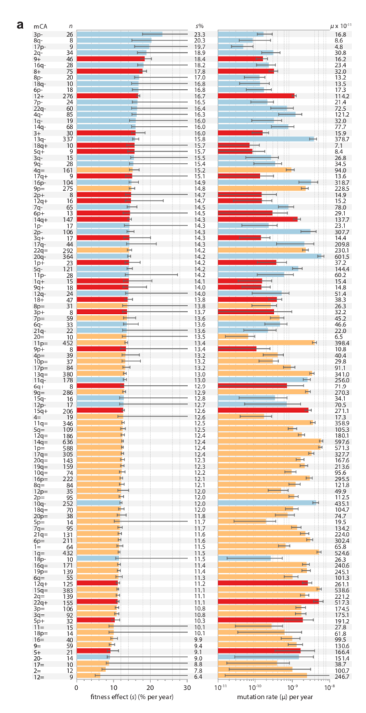
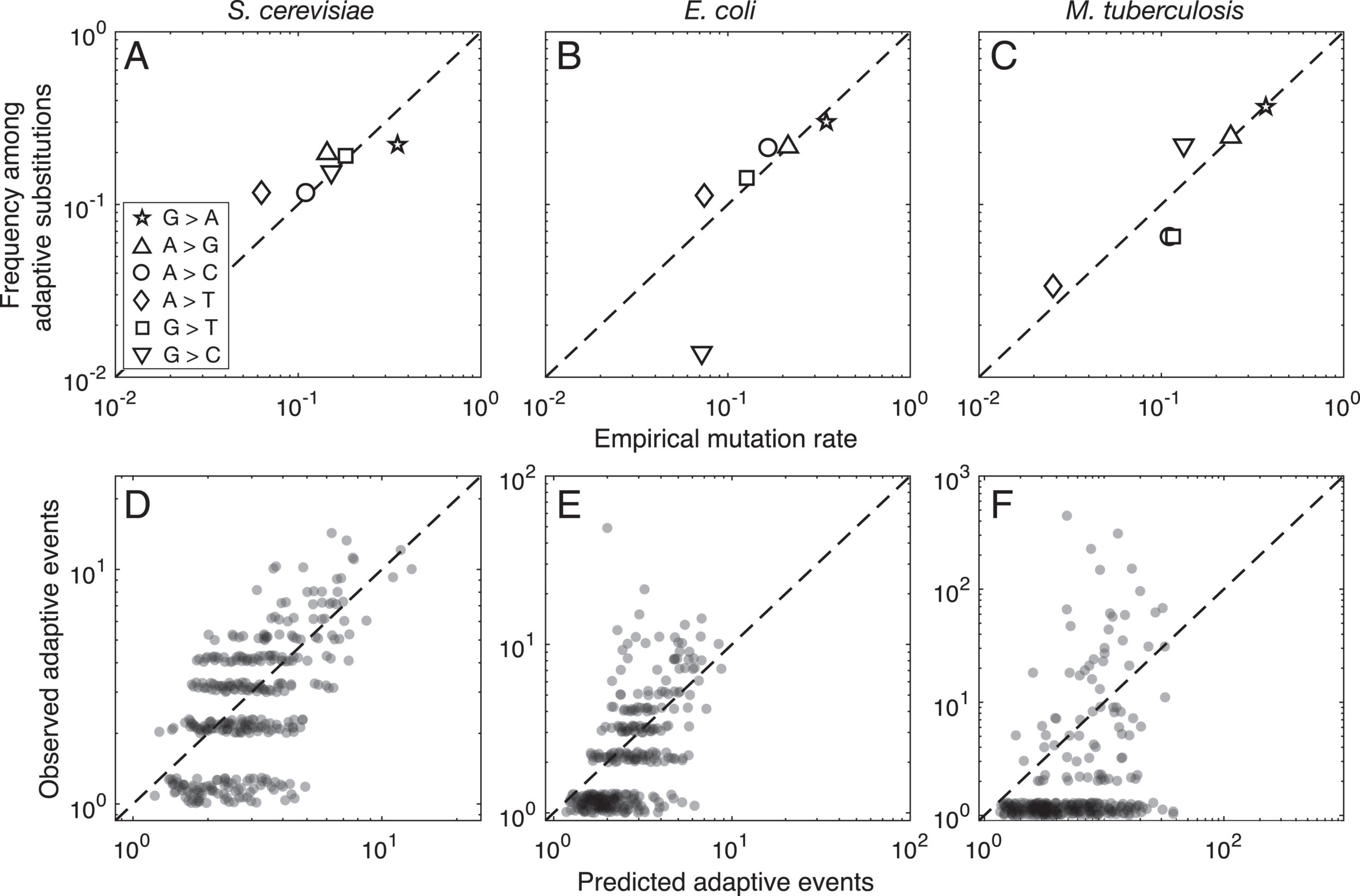
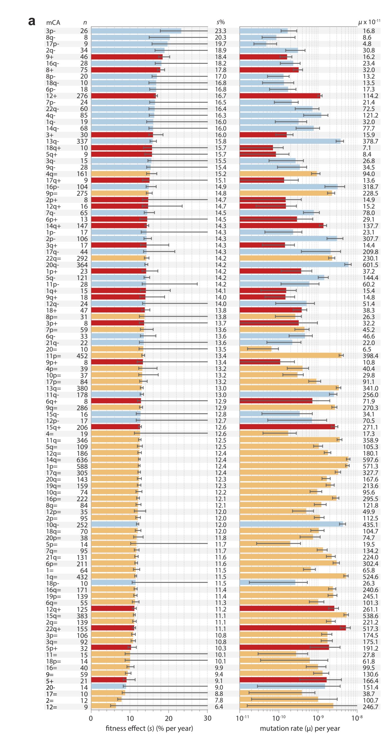
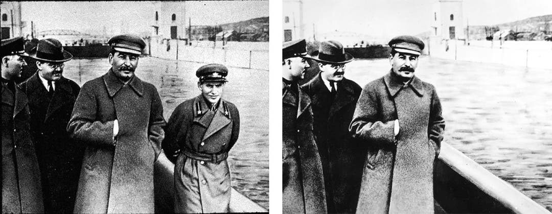


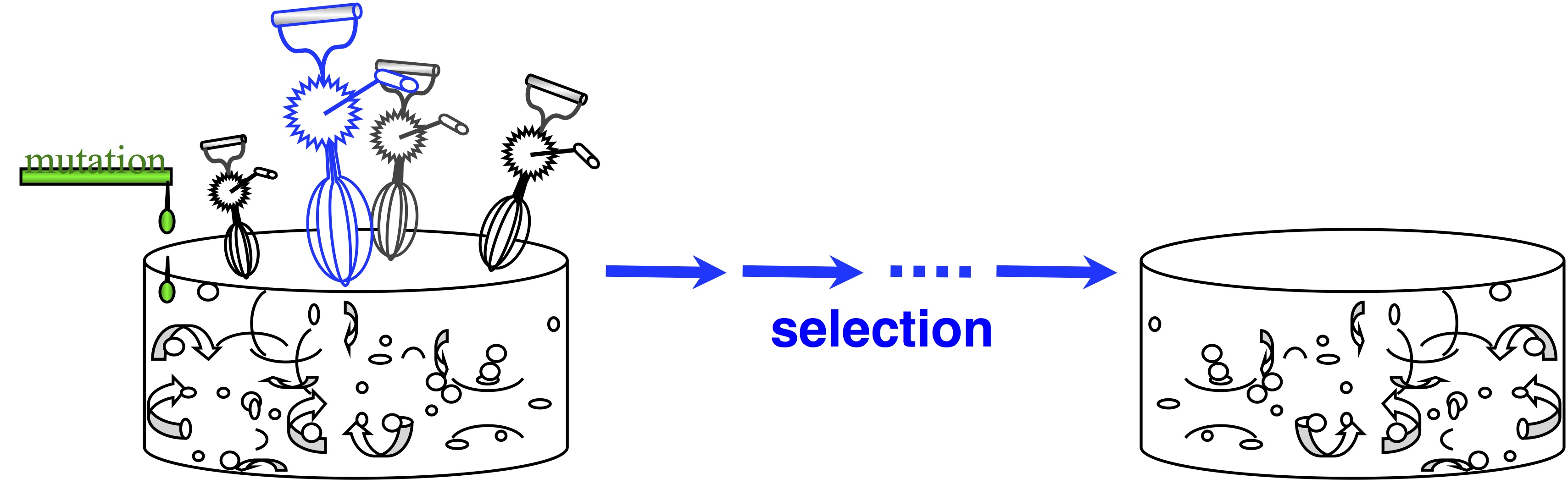
 Note two things about this idea. The first is that this is a modeling assumption, not a feature of reality. Mutations that change 2 sites at once actually occur, and presumably they sometimes contribute to evolution. The second thing to note is that we could choose to define the horizon however we want, e.g., we could include single and double changes, but not triple ones. In practice, the mutational neighbors of a sequence are always defined as the sequences that differ by just 1 residue.
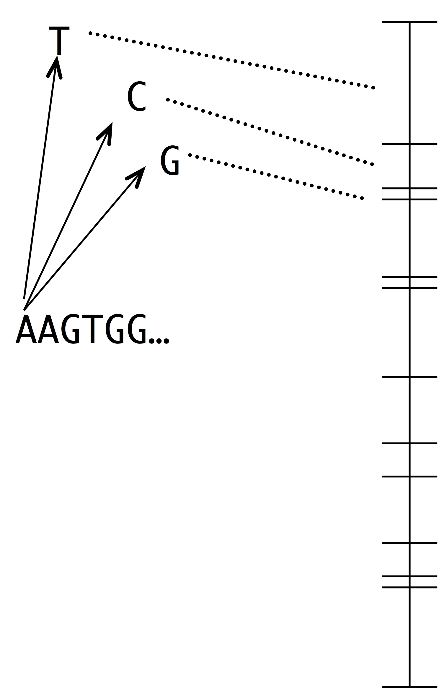
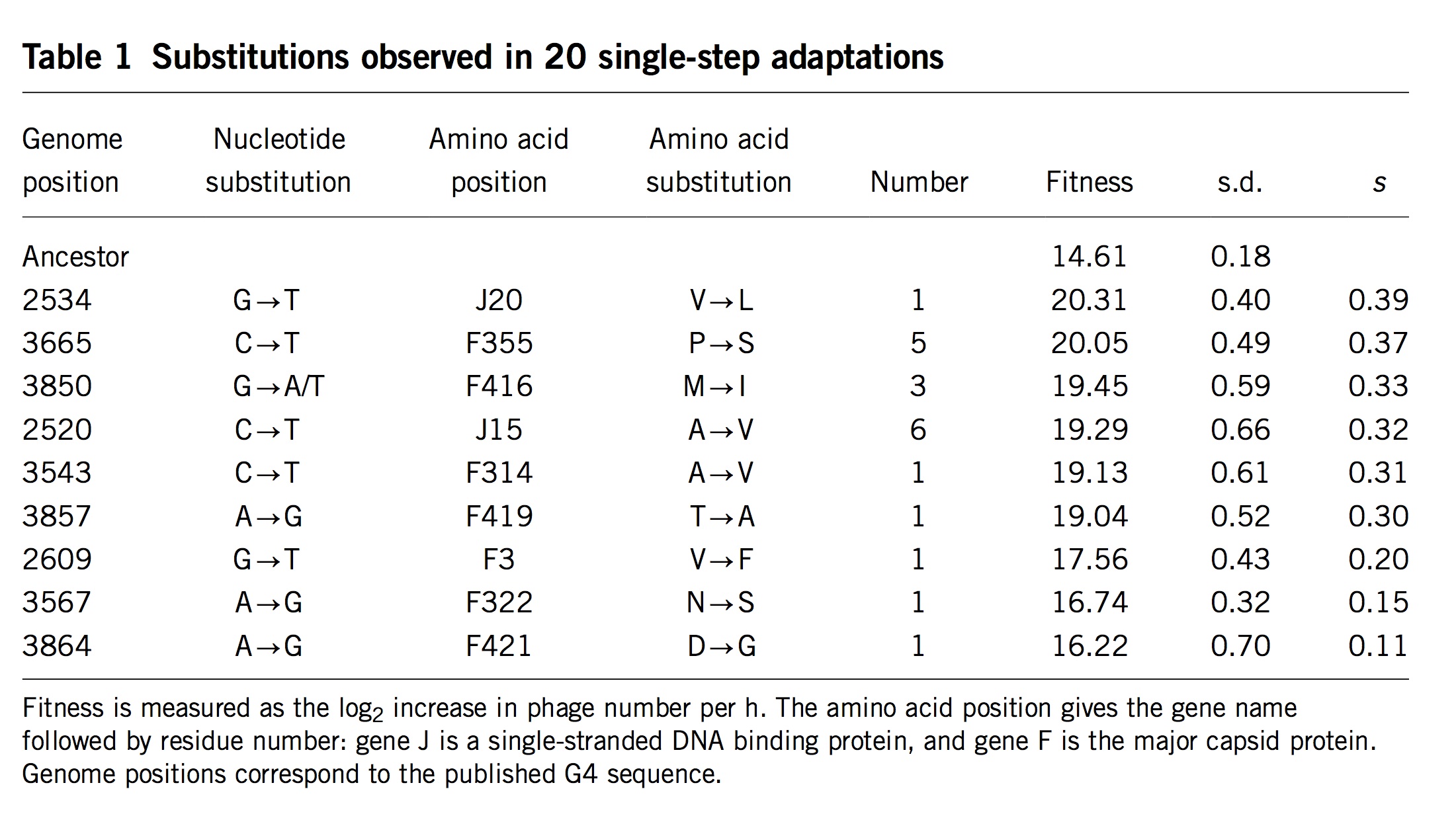
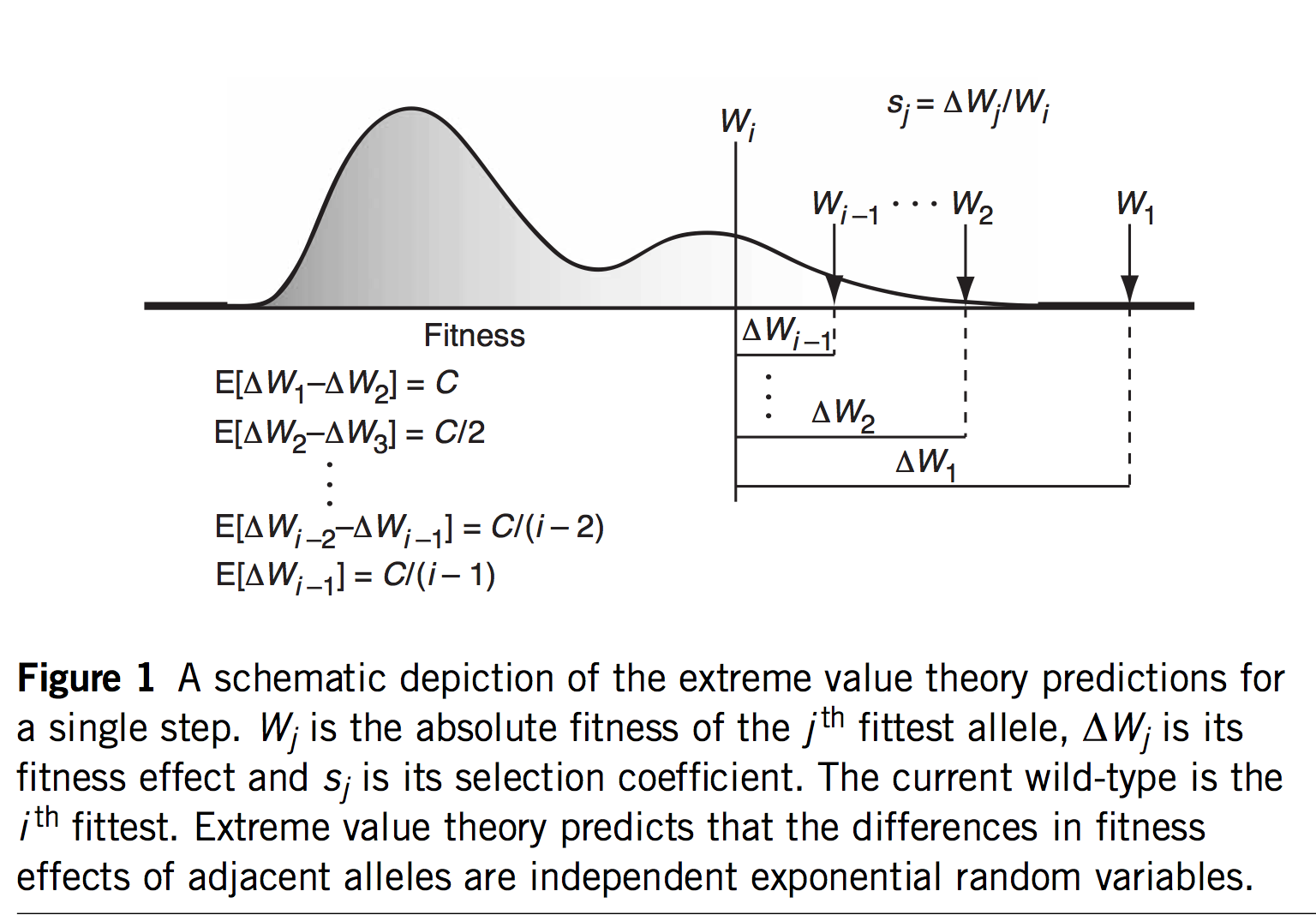
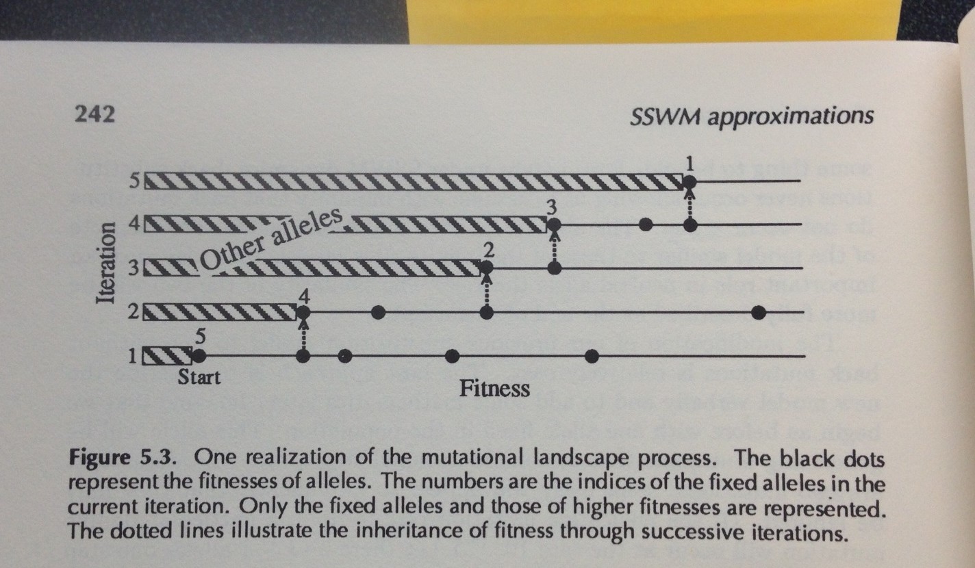
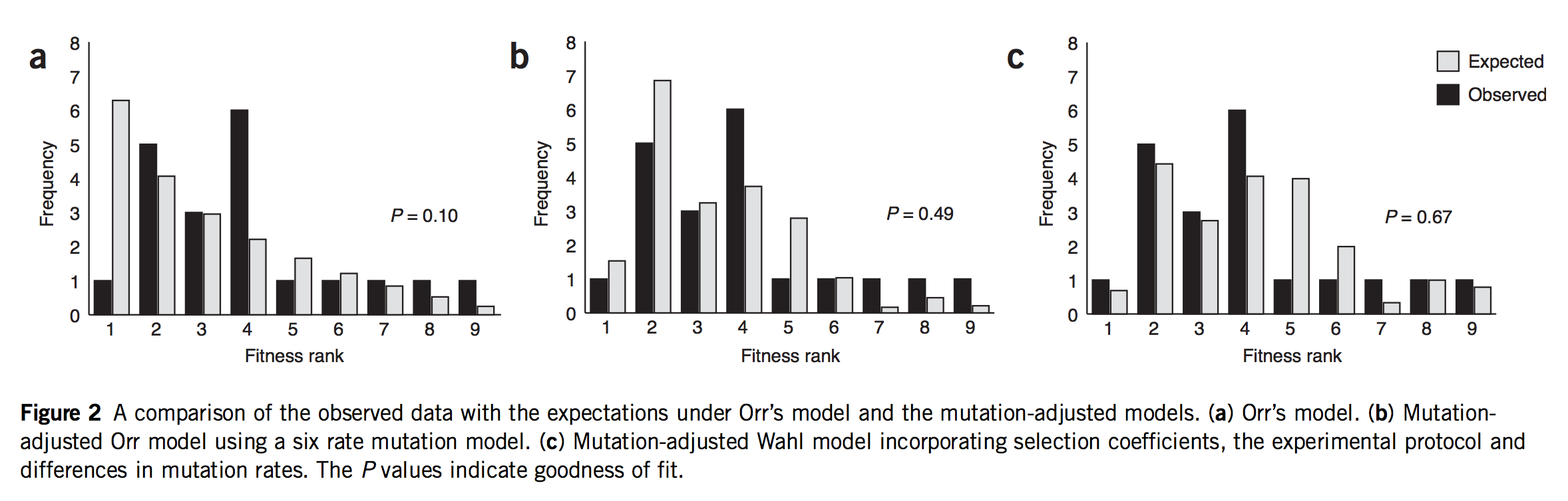
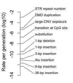


.jpg)
