Some comments on Pachter’s P value prize
In late May, Lior Pachter posted a blog entitled Pachter’s P-value prize, offering a cash prize for providing a probability calculation (P value) based on a “justifiable” null model for the claim of Kellis, Birren and Lander, 2004, hereafter KBL, that some results from an analysis of yeast duplicate genes “strikingly” favored the classic neo-functionalization model of Ohno over the contemporary DDC (duplication-degeneration-complementation) model.
This attracted, not just a huge number of views (for a geeky science blog), but an extensive online discussion among readers that was carried out at a very high intellectual level. Dozens of scientists commented on the blog, including Manolis Kellis, the first author of KBL, and scientists well known in the field of comparative genome analysis. Mostly they were discussing what was an appropriate statistical test, but they also discussed the nature of the Ohno and DDC models, the responsibilities of authors, the flaws of the peer-review process, the appropriateness of blogging and tweeting about science, and so on.
Here, I’m going to use graphics and simulated data to illustrate null models in relation to the duplicate gene data from KBL. I also want to make a comment about the expectations of the DDC model. All of the plots and calculations are available as embedded R code in the R-Markdown file kbl_stats.Rmd.
The data and the challenge
The challenge by Pachter is given as follows:
The authors identified 457 duplicated gene pairs that arose by whole genome duplication (for a total of 914 genes) in yeast. Of the 457 pairs 76 showed accelerated (protein) evolution in S. cerevisiae. The term “accelerated” was defined to relate to amino acid substitution rates in S. cerevisiae, which were required to be 50% faster than those in another yeast species, K. waltii. Of the 76 genes, only four pairs were accelerated in both paralogs. Therefore 72 gene pairs showed acceleration in only one paralog (72/76 = 95%).
So, is it indeed “striking” that “in nearly every case (95%), accelerated evolution was confined to only one of the two praralogues”? Well, the authors don’t provide a p–value in their paper, nor do they propose a null model with respect to which the question makes sense. So I am offering a prize to help crowdsource what should have been an exercise undertaken by the authors, or if not a requirement demanded by the referees. To incentivize people in the right direction, I will award $100/p to the person who can best justify a reasonable null model, together with a p-value (p).
The data underlying the challenge are given in the table below. Is the observation of asymmetric acceleration in 72 of 76 pairs “striking” evidence for Ohno’s model?
| category | count |
| one accelerated | 72 |
| both accelerated | 4 |
| unaccelerated | 381 |
| all | 457 |
Why this isn’t about DDC vs. Ohno
Before addressing Pachter’s challenge, I want to point out the reasons that the results of KBL do not distinguish DDC from Ohno. First, all of this analysis of symmetric vs. asymmetric acceleration is in regard to accelerated rates of change in protein-coding regions. Yet, the most familiar application of the DDC idea is in terms of degeneration and complementation among upstream regulatory modules.
More importantly, the DDC model does not predict symmetric acceleration.
To understand why, it is helpful to consider the little-known quantitative version of sub-functionalization. Of the two 1999 papers that proposed DDC, each paper explicitly presented both a “quantitative” and “qualitative” version: Stoltzfus, 1999 emphasized the quantitative model, while Force, Lynch and colleagues emphasized the qualitative model. The quantitative model can be expressed in terms of a simple scalar quantity, gene activity (i.e., expression multiplied by specific activity). The initial duplication creates 2X activity, but only 1X is required. Thus, copy A can undergo fixation of a neutral mutation that decreases its activity from 1X to 0.6X (for instance). Then if copy B fixes a neutral mutation with a reduction from 1X to 0.5X, we now have 2 genes with a total activity of 1.1X. Neither copy can get lost, because the total activity would drop below 1X. That is, the duplicates are preserved by a neutral model of quantitative sub-functionalization. The reductions can be at the level of gene expression, protein expression, or protein activity.
Prior to the first change in a fresh pair of duplicates, each copy is equally expendable and has the same expected rate of evolution.
However, this period of hypothetical equality ends the moment one copy gets the first hit: then the expected rate of evolution in the other copy drops. For instance, if copy A gets knocked down to 65 % activity, the rate of evolution in copy B is reduced, because it must maintain at least 35 % activity in order for the pair to suffice. Calculating an exact expectation for asymmetry will require a quantitative model of mutational effects, and is complicated by the bifurcation that leads to loss or persistence. The asymmetry presumably will depend strongly on the expected magnitude of the first fixed mutation.
In the qualitative sub-functionalization model, one may suppose that there are n different “functions”: when k of them are compromised in copy A, the evolution of copy B is constrained to preserve the remaining n – k functions. Thus, in the qualitative model, we also expect an asymmetry that depends on the magnitude of the initial effect. This was pointed out by He and Zhang (2005), in response to KBL (here “NF” and “SF” mean neo-functionalization and sub-functionalization):
For example, asymmetric evolutionary rates between duplicates have been used to support NF (KELLIS et al. 2004). But this observation can also be explained by asymmetric SF because the two daughter genes could have inherited different numbers of ancestral functions and thus could be under different levels of functional constraint.
As an aside, I pointed out in 1999 that classic isozyme electrophoresis data from the 1960s and 1970s often shows a pattern in which one duplicate isozyme is consistently lower in activity than the other, across a range of tissues. In the article by Lan and Pritchard that is the initial topic of Pachter’s blog, the authors point out a similar pattern in gene expression data.
To reiterate, this is not an analysis of Ohno vs. DDC. It is an analysis of symmetric vs. asymmetric acceleration. Even if we can sort out the best statistical way to distinguish these two, the distinction does not map cleanly to models of duplicate gene retention.
Expectations under the two most obvious null models
To understand what is potentially “striking” about a result, one has to understand what is expected. What is expected depends on prior beliefs. In the world of science, populated by skeptics and cynics, the prior belief is some kind of null model in which nothing interesting or important is happening. What is the dullest model for the distribution of symmetric and asymmetric pairs?
Uncorrelated rates
Many of the commentators on the blog calculated expectations under a null model that treats all genes independently, and in which there is no phenomenon of acceleration in a subset of genes, but only an arbitrary choice of the most extreme deviates. The duplicate genes are treated as if 914 genes were drawn from a larger pool and paired up at random to make 457 pairs. If the per-gene chance of acceleration is p, then for a randomly drawn pair of genes, the chances are just like standard Hardy-Weinberg expectations for diploid genotypes: the chance that both will be accelerated is p2, the chance of 1 accelerated is 2p(1 – p), and the chance of neither accelerated is (1 – p)2.
KBL observed 457 * 2 = 914 genes, and 72 + (4 * 2) = 80 of them were accelerated. Thus, the per-gene rate of acceleration is p = 80/914 = 0.0875, and the match between expected and observed values for 457 randomly drawn pairs is:
- both accelerated: p2 = 0.007661, expect 3.501 pairs, observe 4 pairs
- one accelerated: 2 * p * (1 – p) = 0.1597, expect 73.00 pairs, observe 72 pairs
- none accelerated: (1 – p)2 = 0.8326, expect pairs 380.5 pairs, observe 381 pairs
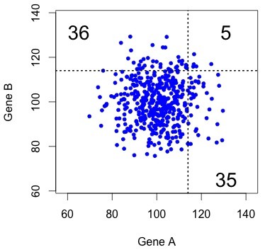
Figure 1. The uncorrelated (independent) null model. Each dot represents a pair, with X and Y coordinates indicating the rates of evolution in copy A and copy B (respectively). The results of KBL are not at all striking under this null model.
There are various ways to calculate a P value for this. The simplest is just a chi-squared test on 3 categories, which gives P = 0.9582. There are more sophisticated ways to do the calculation, but they all give values > 0.5, i.e., they don’t justify the “strikingly” claim of KBL.
This kind of result is very easy to visualize, as in the figure at right. This shows simulated data for 457 pairs of genes, with the rate for gene B plotted as a function of the rate for gene A. The dotted lines show the threshold that gives exactly 76 accelerated pairs. The “both accelerated” pairs are in the upper right quadrant, and the “one accelerated” pairs are in the lower right and upper left.
Typically there are only a few dots in the “both accelerated” quadrant. That is, under this null model, the results of KBL are trivial.
Correlated rates
Kellis objected that this null model of uncorrelated genes is unreasonable. Even if duplicate genes evolve independently after duplication, we do not expect them to have uncorrelated rates. Members of some gene families consistently evolve at lower rates than others, e.g., histones evolve more slowly than globins.
So, what is a reasonable null model for correlated evolution? Let us assign each gene pair a stochastic deviation in underlying rate, including deceleration and acceleration.
It turns out that we cannot define a null model without making critical assumptions about the correlation. The reason is shown in the set of plots below. When the correlation is very weak (upper left), results are similar to the uncorrelated case (above), for which the numbers strongly favor “one accelerated”. As the correlation gets stronger (below right), the numbers strongly favor “both accelerated”.

Figure 2. The correlated null model, shown for a range of correlations in 457 pairs. Each dot represents a gene pair, as in Figure 1. In this case, the rates are correlated. The underlying rates for families are normal with mean 100 and sd 10, and the members of a pair have deviations (from the family’s underlying rate) with a mean of 0 and a standard deviation ranging from 16 to 1. Similar results are observed from a model that uses a constant coefficient of variation (i.e., the deviation is scaled to the family-specific rate, so that faster families have more within-family deviation).
How can we test for a deviation from a null model of correlated rates? I can’t think of a way to do this non-parametrically, because each gene pair has a characteristic underlying rate, and a stochastic between-copy divergence, and we can’t separate those two effects without introducing some scaling assumptions. Presumably, to devise a test, we would have to assume (1) a particular shape for the underlying distribution of family rates, and (2) a model of within-family deviations. In the examples above, they are both normally distributed.
What was the implicit KBL model?
As noted, KBL do not report a P value, nor describe a null model. Kellis explains that KBL are just comparing two numbers to see which is bigger, in order to determine which model is more important. That is, they find that 72 is bigger than 4, and conclude from this that Ohno’s model is far more important than DDC (e.g., by a binomial test, p < 2 X 10-16). It took me a long time to realize that this is what KBL were thinking, although Erik van Nimwegen pointed this out in his comments on Pachter’s blog.
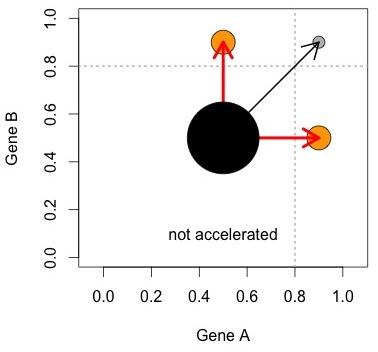
Figure 3. An attempt to make sense out of what KBL did. See text for explanation
The figure at right helps to visualize the logic. The Ohno process, represented by the red arrows, results in asymmetrically accelerated pairs. Some other process (black arrow) creates symmetrically accelerated pairs. The null model is that the two processes are equally important. This can be evaluated with a simple comparison of numbers of pairs (size of orange circles vs. grey circle).
In this hypothetical world, there are exactly 2 processes, and each creates its own unique category. Figures 1 and 2 show why we can’t trust this simplistic view: we can create a range of possible outcomes— from a strong bias toward symmetric pairs, to a strong bias toward asymmetric pairs— just by manipulating (1) stochastic rate differences and (2) within-pair correlation of rates, and without including either the Ohno process or the DDC process.
I wanna be a millionaire
When Pachter offered his prize of $100/p, he seems to have been assuming that the only “justifiable” null model would be the independent model, which has a P value close to 1. Thus, he did not expect to pay out more than $200.
The problem with Pachter’s assumption is that one does not have to accept the independent model as a reasonable null model. Members of different gene families evolve at systematically different rates. As noted above, we can’t test for deviation from the correlated-rates model without information that Pachter’s challenge does not supply.
So, what do the data actually look like? To see the actual distribution, you need to download the Duplicated Pairs.xls spreadsheet from Kellis’s web site. Some transformation is needed to convert this into relative rate data comparable to the simulated data above (see the R code mentioned earlier). 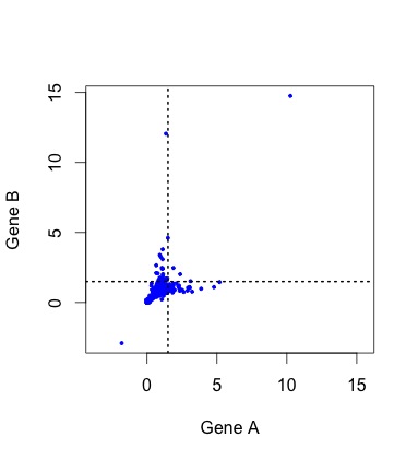 When we do this, there are a handful of negative values (?!?) and a couple of outliers that make it hard to see the pattern clearly (small figure, left). In the larger figure (below, right), I have discarded these (which discards 1 of the 4 lonely points in the “symmetric acceleration” quadrant). The rates are expressed relative to control rates in the outgroup subtree (K. waltii), thus the mass is centered around (1, 1).
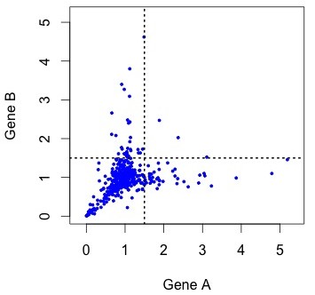
Figure 4. KBL rate data for ~450 pairs of duplicate genes, where the assignment to A or B has been randomized to make it comparable to earlier figures. The rates are relative to the rate of evolution of homologs in K. waltii.
As you can see, the rates are strongly correlated. The correlation is about R2 = 0.33 for all the data, and R2 = 0.63 for the unaccelerated pairs in the lower left quadrant. However, the gene pairs seem to be avoiding the upper right quadrant. The diagonal “Y” pattern is more of an asymmetry than an anti-correlation: higher-than-average rates for one gene are paired with average rates for the other, as if the acceleration of one gene were independent of its partner.
How significant is that pattern? As a very simple conservative test, let’s take the conditions from panel 9 of Figure 2, which has a similar degree of correlation as the entire distribution, simulate 10,000 replicates, and ask how often we would find such a high proportion of asymmetric pairs as 72 out of 76. We are just trying to get a feel for how extreme is the pattern in Figure 4 relative to a null model.
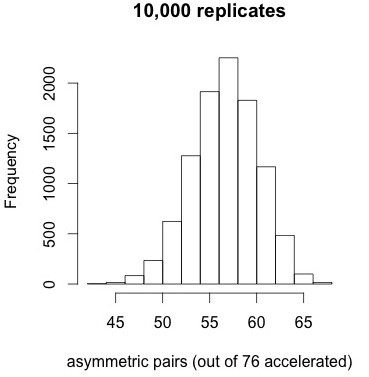
Figure 5. Results of 10,000 simulations under the correlated null model do not reveal any replicates with 72 or more asymmetric pairs (when 76 pairs out of 453 are accelerated).
This is a conservative test because I am picking the low end of the correlation. If we did the test based on R2 = 0.63, which looks more like panel 12 of Figure 2, the deviation from the null model would be even more extreme.
The results shown at left indicate that the tendency for accelerated pairs to be asymmetric is very striking under the correlated null model. No replicates out of 10,000 have 72 or more accelerated pairs, i.e., apparently p < 1e-4. The mean is about 57 and the standard deviation is about 3.5. Too bad this result doesn’t help us to distinguish models of duplicate gene evolution. It just tells us that when duplicate genes show accelerated evolution, the asymmetry is extreme.
Caveat emptor
Note that my statistics above are crude. Even if they were more sophisticated, I don’t think this is the end of the discussion on how best to analyze these data. None of the above tests are very good because we are doing them on normalized rate estimators rather than directly on observations (e.g., counts of changed residues between paralogs). If one is working with actual counts, and the numbers are small, strange things can happen even in a null model.
Lessons learned
What did I learn from this?
First of all, folks, we really need to think more carefully about evolutionary models and what they imply. This whole debacle has no clear relationship to distinguishing Ohno and DDC. As Matt Hahn pointed out in the online discussion, we only have vague intuitive expectations, not formal and precise expectations, for what the pattern of duplicate gene divergence should look like. The population-genetics underlying DDC lead to some expectations about the relationship to population size. That’s not much— not much leverage to test hypotheses or make inferences. This is a challenge for theoretical work, not data analysis. Further data analysis without clear expectations is a misallocation of scientific effort. Please, stop.
Second, it is important to specify and test null models, even simplistic ones. Perhaps the uncorrelated model is unrealistic. Perhaps the correlated model also is unrealistic. However, I do not think null models should be ruled out a priori based on being unrealistic. I think there is an important place in science for testing idealized unrealistic models.
Third, science is complicated. Yes, obviously, we expect key claims based on the analysis of numeric data to be accompanied by an explicit calculation indicating significance. The KBL paper is flawed in this regard. However, when one looks at the actual KBL data, we can reject the uncorrelated null model, because the rates clearly are correlated, and we can reject the correlated null model, because of the excess asymmetry in the upper part of the distribution. It may be an artifact of data processing, and sadly it has little to tell us about models of gene duplication, but it is an interesting pattern that deserves an explanation.
BTW, I entered this contest late, so I’m not going to be demanding the $100/p > $1e6 from Pachter.
Pinko Punko
June 19, 2015 - 12:24 am
Would it also be fair to assume that duplications arising from whole genome duplication complicates the analysis of understanding how genes evolve subsequent to duplication?
Arlin Stoltzfus
June 19, 2015 - 1:38 am
Yes, absolutely. One complication this introduces is the potential emergence of reproductive isolation due to reciprocal gene losses, an idea attributed to Oka. Probably there are other complications. My calculations here assume that all gene families (gene pairs) are independent.