October 2, 2015 / Arlin Stoltzfus / 0 Comments
This post started out as a wonky rant about why a particular high-profile study of laboratory adaptation was mis-framed as though it were a validation of the mutational landscape model of Orr and Gillespie (see Orr, 2003), when in fact the specific innovations of that theory were either rejected, or not tested critically. As I continued ranting, I realized that there was quite a bit to say that is educational, and I contemplated that the reason for the original mis-framing is that this is an unfamiliar area, such that even the experts are confused— which means that there is a value to explaining things.
The crux of the matter is that the Gillespie-Orr “mutational landscape” model has some innovations, but also draws on other concepts and older work. We’ll start with these older foundations.
Origin-fixation dynamics in sequence space
First, the mutational landscape model draws on origin-fixation dynamics, proposed in 1969 by Kimura and Maruyama, and by King and Jukes (see McCandlish and Stoltzfus for an exhaustive review, or my blog on The surprising case of origin-fixation models).
In origin-fixation models, evolution is seen as a simple 2-step process of the introduction of a new allele, and its subsequent fixation (image).  The rate of change is then characterized as a product of 2 factors, the rate of mutational origin (introduction) of new alleles of a particular type, and the probability that a new allele of that type will reach fixation. Under some general assumptions, this product is equal to the rate of an origin-fixation process when it reaches steady state.
Probably the most famous origin-fixation model is K = 4Nus, which uses 2s (Haldane, 1927) for the probability of fixation of a beneficial allele, and 2Nu (diploids) for the rate of mutational origin. Thus K = 4Nus is the expected rate of changes when we are considering types of beneficial alleles that arise by mutation at rate u, and have a selective advantage s. But we can adapt origin-fixation dynamics to other cases, including neutral and deleterious changes. If we were applying origin-fixation dynamics to meiotic bursts, or to phage bursts, in which the same mutational event gives rise immediately to multiple copies (prior to selection), we would use a probability of fixation that takes this multiplicity into account.
In passing, note that origin-fixation models appeared in 1969, and we haven’t always viewed evolution this way. The architects of the Modern Synthesis rejected this view— and if you don’t believe that, read The Shift to Mutationism is Documented in Our Language or The Buffet and the Sushi Conveyor. They saw evolution as more of an ongoing process of “shifting gene frequencies” in a super-abundant “gene pool” (image). 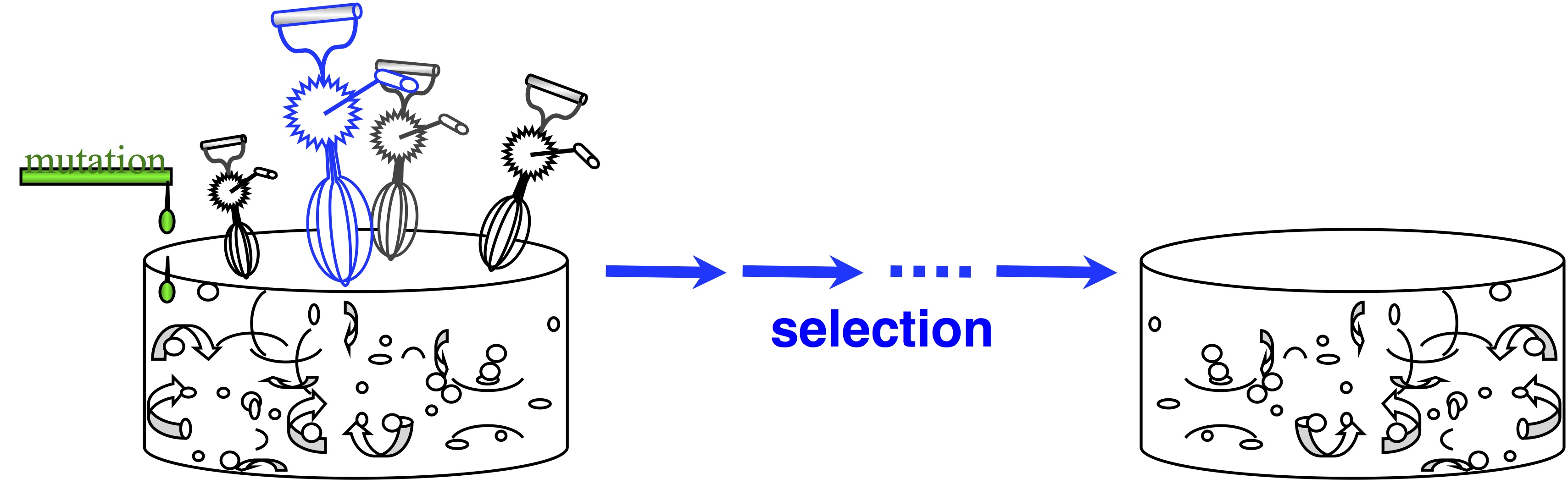 Mutation merely supplies variation to the “gene pool”, which is kept full of variation. The contribution of mutation is trivial. The available variation is constantly mixed up by recombination, represented by the egg-beaters in the figure. When the environment changes, selection results in a new distribution of allele frequencies, and that’s “evolution”— shifting gene frequencies to a new optimum in response to a change in conditions.
This is probably too geeky to mention, but from a theoretical perspective, an origin-fixation model might mean 2 different things. It might be an aggregate rate of change across many sites, or the rate applied to a sequence of changes at a single locus. The mathematical derivation, the underlying assumptions, and the legitimate uses are different under these two conditions, as pointed out by McCandlish and Stoltzfus. The early models of King, et al were aggregate-rate models, while Gillespie, (1983) was the first to derive a sequential-fixations model.
Second, the mutational landscape model draws on Maynard Smith’s (1970) concept of evolution as discrete stepwise movement in a discrete “sequence space”. More specifically, it draws on the rarely articulated locality assumption by which we say that a step is limited to mutational “neighbors” of a sequence that differ by one simple mutation, rather than the entire universe of sequences. The justification for this assumption is that double-mutants, for instance, will arise in proportion to the square of the mutation rate, which is a very small number, so that we can ignore them. Instead, we can think of the evolutionary process as accessing only a local part of the universe of sequences, which shifts with each step it takes. In order for adaptive evolution to happen, there must be fitter genotypes in the neighborhood.
This is an important concept, and we ought to have a name for it. I call it the “evolutionary horizon”, because we can’t see beyond the horizon, and the horizon changes as we move.  Note two things about this idea. The first is that this is a modeling assumption, not a feature of reality. Mutations that change 2 sites at once actually occur, and presumably they sometimes contribute to evolution. The second thing to note is that we could choose to define the horizon however we want, e.g., we could include single and double changes, but not triple ones. In practice, the mutational neighbors of a sequence are always defined as the sequences that differ by just 1 residue.
Putting these 2 pieces together, we can formulate a model of stepwise evolution with predictable dynamics.
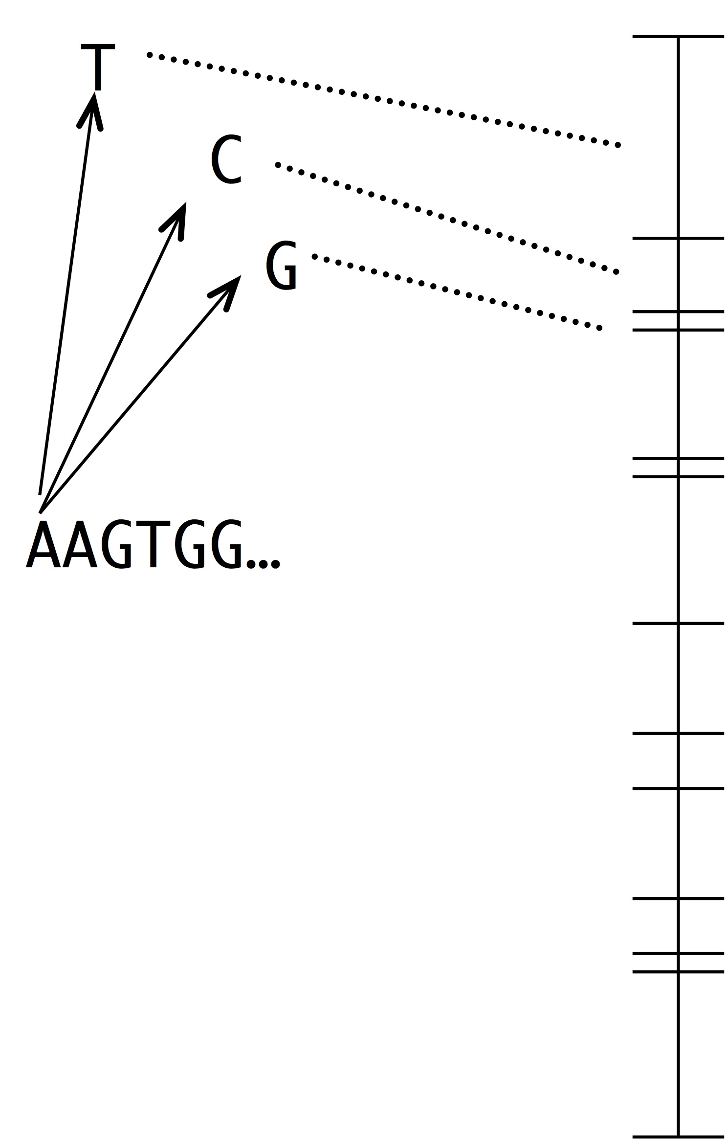 Making this into a simulation of evolution is easy using the kind of number line shown at left. Each segment represents a possible mutation-fixation event from the starting sequence. For instance, we can change the “A” nucleotide that begins the sequence to “T”, “C” or “G”. The length of each segment is proportional to the origin-fixation probability for that change (where the probability is computed from the instantaneous rate). To pick the next step in evolution, we simply pick a random point on the number line. Then, we have to update the horizon— recompute the numberline with the new set of 1-mutant neighbors.
Where do we get the actual values for mutation and fixation? One way to do it is by drawing from some random distribution. I did this in a 2006 simulation study. I wasn’t doing anything special. It seemed very obvious at the time.
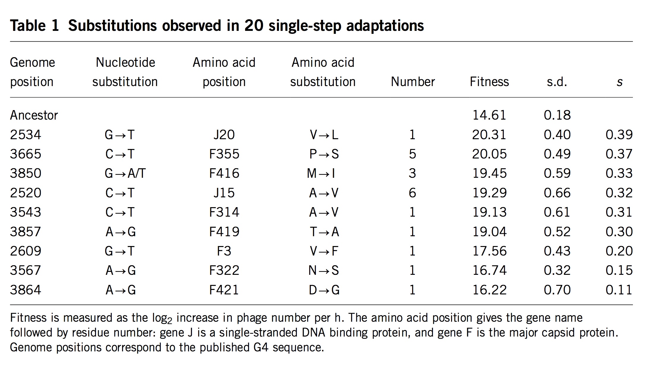
(Table 1 from Rokyta, et al)
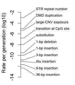
Surprisingly, researchers almost never measure actual mutation and selection values for relevant mutants. One exception is the important study by Rokyta, et al (2005), who repeatedly carried out 1-step adaptation using bacteriophage phiX174. The selection coefficients for each of the 11 beneficial changes observed in replicate experiments are shown in the rightmost column, with the mutants ranked from highest to lowest selection coefficient. Notice that the genotype that recurred most often (see the “Number” column) was not the alternative genotype with the highest fitness, but the 4th-most-fit alternative, which happened to be favored by a considerable bias in mutation. Rokyta, et al didn’t actually measure specific rates for each mutation, but simply estimated average rates for different classes of nucleotide mutation based on an evolutionary model.
Then Rokyta, et al. developed a model of origin-fixation dynamics using the estimated mutation rates, the measured selection coefficients, and a term for the probability of fixation customized to account for the way that phages grow. This model fit the data very well, as I’ll show in a figure below (panel C in the final figure).
The mutational landscape model
Given all of that, you might ask, what does the mutational landscape model do?
This is where the specific innovations of Orr and Gillespie come in. Just putting together origin-fixation dynamics and an evolutionary horizon doesn’t get us very far, because we can’t actually predict anything without filling in something concrete about the parameters, and that is a huge unknown. What if we don’t have that? Furthermore, although Rokyta, et al implicitly assumed a horizon in the sense that they ignored mutations too rare to appear in their study, they never tackled the question of how the horizon shifts with each step, because they only took one step. What if we want to do an extended adaptive walk? How will we know what is the distribution of fitnesses for the new set of neighbors, and how it relates to the previous distribution? In the simulation model that I mentioned previously, I used an abstract “NK” model of the fitness of a protein sequence that allowed me to specify the fitness of every possible sequence with a relatively small number of randomly assigned parameter values.
Gillespie and Orr were aiming to do something more clever than that. Theoreticians want to find ways to show something interesting just from applying basic principles, without having to use case-specific values for empirical parameters. After all, if we insert the numbers from one particular experimental system, then we are making a model just for that system.
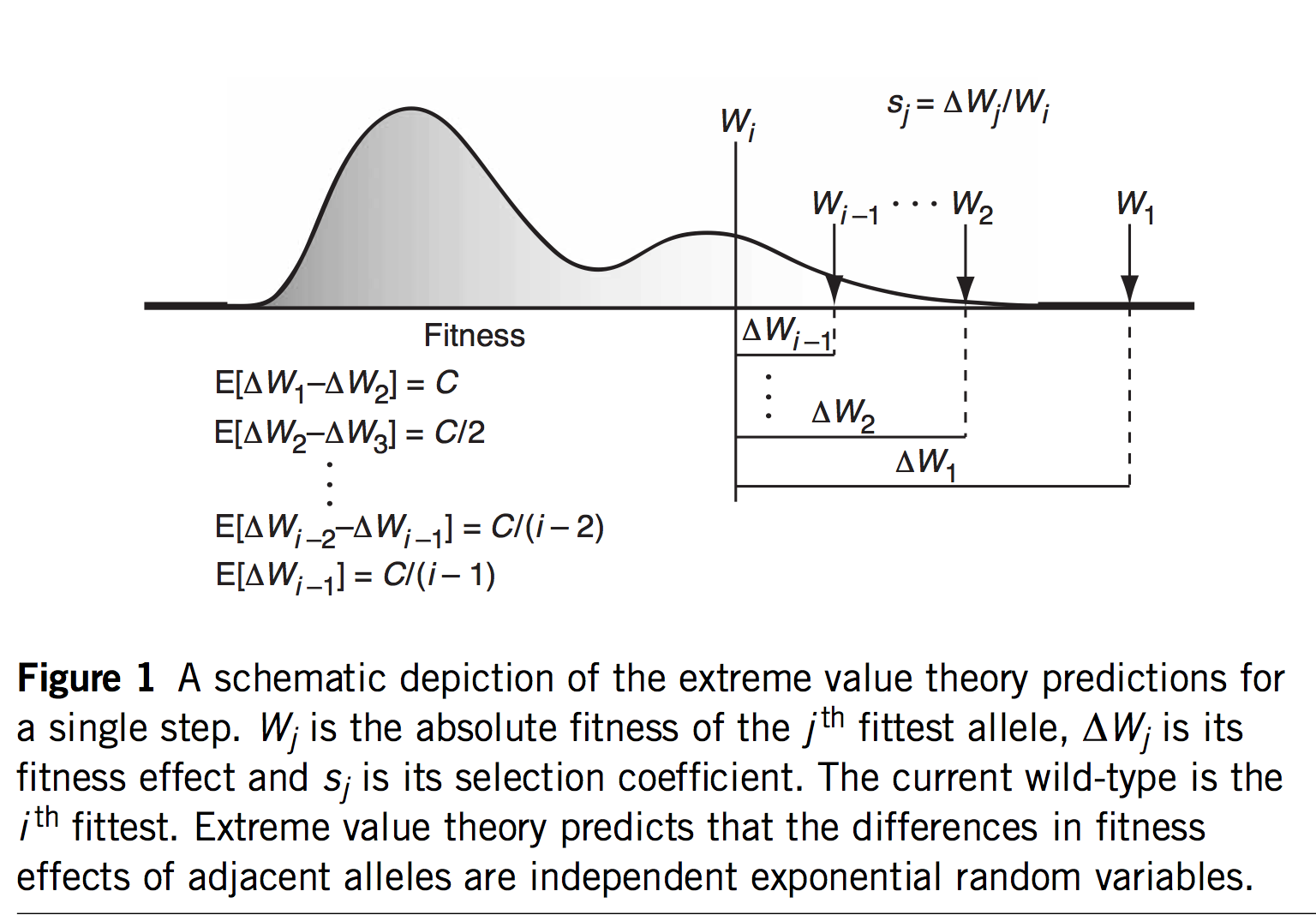
(Figure 1 of Rokyta, et al, explaining EVT)
The first innovation of Orr and Gillespie is to apply extreme value theory (EVT) in a way that offers predictions even if we haven’t measured the s values or assumed a specific model. If we assume that the current genotype is already highly adapted, this is tantamount to assuming it is in the tail end of a fitness distribution. EVT applies to the tail ends of distributions, even if we don’t know the specific shape of the distribution, which is very useful. Specifically, EVT tells us something about the relative sizes of s as we go from one rank to the next among the top-ranked genotypes: the distribution of fitness intervals is exponential. This leads to very specific predictions about the probability of jumping from rank r to some higher rank r’, including a fascinating invariance property where the expected upward jump in the fitness ranking is the same no matter where we are in the ranking. Namely, if the rank of the current genotype is j (i.e., j – 1 genotypes are better), we will jump to rank (j + 2)/4.
That’s fascinating, but what are we going to do with that information? I suspect the idea of a fitness rank previously appeared nowhere in the history of experimental biology, because rank isn’t a measurement one takes anywhere other than the racetrack. But remember that we would like a theory for an adaptive walk, not just 1-step adaptation. If we jump from j to k = (j + 2)/4, then from k to m = (k + 2)/4, and so on, we could develop a theory for the trajectory of fitness increases during an adaptive walk, and for the length of an adaptive walk— for how many steps we are likely to take before we can’t climb anymore.
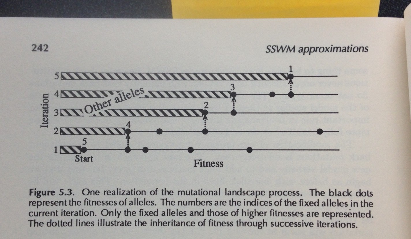
Figure 5.3 from Gillespie’s 1991 book. Each iteration has a number-line showing the higher-fitness genotypes accessible on the evolutionary horizon (fitness increases going to the right). At iteration #1, there are 4 more-fit genotypes. In the final iteration, there are no more-fit genotypes accessible, but there is a non-accessible more-fit genotype that was accessible at iteration #2.
The barrier to solving that theory is solving the evolutionary horizon problem. Every time we take a step, the horizon shifts— some points disappear from view, and others appear (Figure). We might be the 15th most-fit genotype, but at any step, only a subset of the 14 better genotypes will be accessible, and this subset changes with each step: this condition is precisely what Gillespie (1984) means by the phrase “the mutational landscape” (see Figure). In his 1983 paper, he just assumes that all the higher-fitness mutants are accessible throughout the walk. Gillespie’s 1984 paper entitled “Molecular Evolution over the Mutational Landscape” tackles the changing horizon explicitly. He doesn’t solve it analytically, but uses simulations. I won’t explain his approach, which I don’t fully understand. Analytical solutions appeared in later work by Jain and Seetharaman, 2011 (thanks to Dave McCandlish for pointing this out).
The third and fourth key innovations are to (3) ignore differences in u and (4) treat the chances of evolution as a linear function of s, based on Haldane’s 2s. In origin-fixation dynamics, the chance of a particular step is based on a simple product: rate of origin multiplied by probability of fixation. Orr’s model relates the chances of an evolutionary step entirely to the probability of fixation, assuming that u is uniform. Then, using 2s for the probability of fixation means that the chance of picking a mutant with fitness si is simply si / sum(s) where the sum is over all mutants (the factor of 2 cancels out because its the same for every mutant). Then, by applying EVT to the distribution of s, the model allows predictions based solely on the current rank.
A test of the mutational landscape model?
As noted earlier, this post started as a rant about a study that was mis-framed as though it were some kind of validation of Orr’s model. In fact, that study is Rokyta, et al., described above. Indeed, Rokyta, et al. tested Orr’s predictions, as shown in the left-most panel in the figure below. The predictions (grey bars) decrease smoothly because they are based, not on the actual measured fitness values shown above, but merely on the ranking. The starting genotype is ranked #10, and all the predictions of Orr’s model follow from that single fact, which is what makes the model cool!
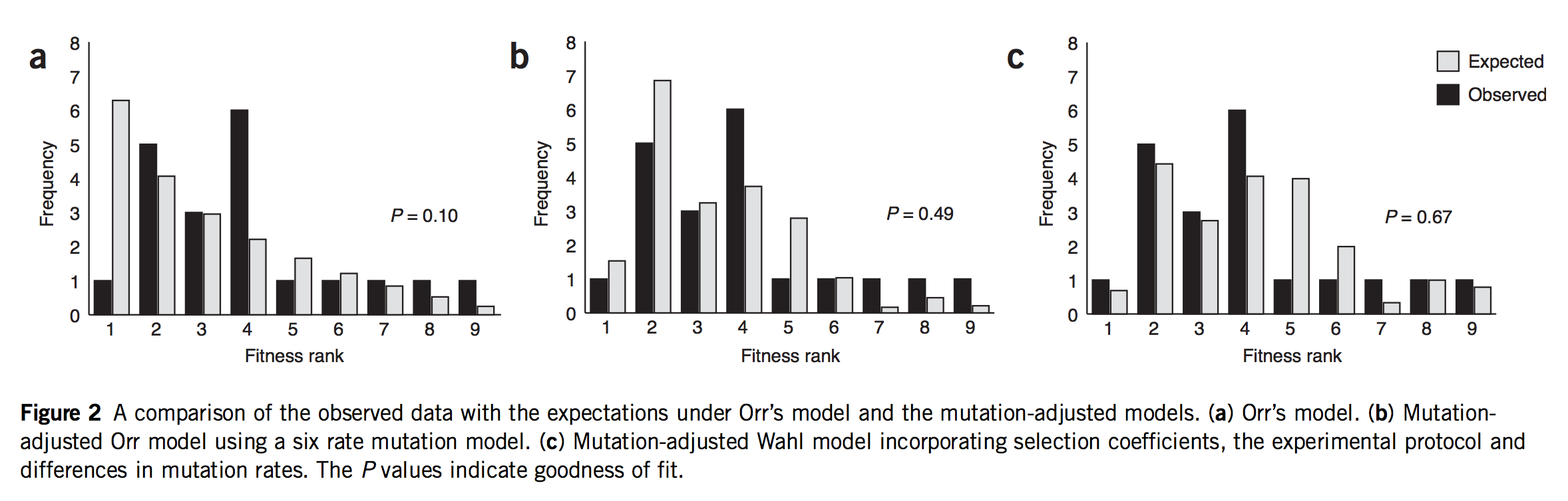
(Figure 2 of Rokyta, et al. A: fit of data to Orr’s model. B: fit of data to an origin-fixation model using non-uniform mutation rates. C: fit of data to origin-fixation model with non-uniform mutation and probability of fixation adjusted to fit phage biology more precisely. The right model is significantly better than the left model.)
If they did a test, what’s my objection? Yes, Rokyta, et al. turned the crank on Orr’s model and got predictions out, and did a goodness-of-fit test comparing observations to predictions. But, to test the mutational landscape model properly, you have to turn the crank at least 2 full turns to get the mojo working. Remember, what Gillespie means by “evolution over the mutational landscape” is literally the way evolution navigates the change in accessibility of higher-fitness genotypes due to the shifting evolutionary horizon. That doesn’t come into play in 1-step adaptation. You have to take at least 2 steps. Claiming to test the mutational landscape model with data on 1-step adaptation is like claiming to test a new model for long-range weather predictions using data from only 1 day.
The second problem is that Rokyta, et al respond to the relatively poor fit of Orr’s model by successively discarding every unique feature. The next thing to go was the assumption of uniform mutation. As I noted earlier, there are strong mutation biases at work. So, in the middle panel of the figure above, they present a prediction that depends on EVT and assumes Haldane’s 2s, but rejects the uniform mutation rate. In their best model (right panel) they have discarded all 4 assumptions. They have measured the fitnesses (Table 1, above), and they aren’t a great fit to an exponential, so they just use these instead of the theory. Haldane’s 2s only works for small values of s like 0.01 or 0.003, but the actual measured fitnesses go from 0.11 to 0.39! Rokyta, et al provide a more appropriate probability of fixation developed by theoretician Lindi Wahl that also takes into account the context of phage (burst-based) replication. To summarize,
Assumption 1 of the MLM. The exponential distribution of fitness among the top-ranked genotypes is tested, but not tested critically, because the data are not sufficient to distinguish different distributions.
Assumption 2 of the MLM. Gillespie’s “mutational landscape” strategy— his model for how the changing horizon cuts off previous choices and offers a new set of choices at each step— isn’t tested because Rokyta’s study is of 1-step walks.
Assumption 3 of the MLM. The assumption that the probability of a step is not dependent on u, on the grounds that u is uniform or inconsequential, is rejected, because u is non-uniform and consequential.
Assumption 4 of the MLM. The assumption that we can rely on Haldane’s 2s is rejected, for 2 different reasons explained earlier.
Conclusion
I’m not objecting so much to what Rokyta, et al wrote, and I’m certainly not objecting to what they did— it’s a fine study, and one that advanced the field. I’m mainly objecting to the way this study is cited by pretty much everyone else in the field, as though it were a critical test that validates Orr’s approach. That just isn’t supported by the results. You can’t really test the mutational landscape model with 1-step walks. Furthermore, the results of Rokyta, et al led them away from the unique assumptions of the model. Their revised model just applies origin-fixation dynamics in a realistic way suited to their experimental system— which has strong mutation biases and special fixation dynamics— and without any of the innovations that Orr and Gillespie reference when they refer to “the mutational landscape model.”